Article

Identifying and Quantifying the Abundance of Economically Important Palms in Tropical Moist Forest Using UAV Imagery

by
Ximena Tagle Casapia
1,2,*,
Lourdes Falen
1,
Harm Bartholomeus
2,
Rodolfo Cárdenas
3,
Gerardo Flores
1,
Martin Herold
2,
Eurídice N. Honorio Coronado
1 and
Timothy R. Baker
4
1
Dirección de Investigación en Manejo Integral del Bosque y Servicios Eco sistémicos - PROBOSQUES, Instituto de Investigaciones de la Amazonía Peruana (IIAP), Av. A. Quiñones Km. 2.5. Iquitos 16007, Peru
2
Laboratory of Geo-Information Science and Remote Sensing, Wageningen University & Research, Droevendaalsesteeg 3, 06708 PB Wageningen, The Netherlands
3
Dirección de Gestión del Conocimiento e Investigación en Información de Diversidad Amazónica - GESCON, Instituto de Investigaciones de la Amazonía Peruana (IIAP), Av. A Quiñones Km. 2.5. Iquitos 16007, Peru
4
School of Geography, University of Leeds, Leeds LS2 9JT, UK
*
Author to whom correspondence should be addressed.
Remote Sens. 2020, 12(1), 9; https://doi.org/10.3390/rs12010009
Submission received: 20 November 2019 / Revised: 11 December 2019 / Accepted: 16 December 2019 / Published: 18 December 2019
(This article belongs to the Section Forest Remote Sensing)

Abstract

:
Sustainable management of non-timber forest products such as palm fruits is crucial for the long-term conservation of intact forest. A major limitation to expanding sustainable management of palms has been the need for precise information about the resources at scales of tens to hundreds of hectares, while typical ground-based surveys only sample small areas. In recent years, small unmanned aerial vehicles (UAVs) have become an important tool for mapping forest areas as they are cheap and easy to transport, and they provide high spatial resolution imagery of remote areas. We developed an object-based classification workflow for RGB UAV imagery which aims to identify and delineate palm tree crowns in the tropical rainforest by combining image processing and GIS functionalities using color and textural information in an integrative way to show one of the potential uses of UAVs in tropical forests. Ten permanent forest plots with 1170 reference palm trees were assessed from October to December 2017. The results indicate that palm tree crowns could be clearly identified and, in some cases, quantified following the workflow. The best results were obtained using the random forest classifier with an 85% overall accuracy and 0.82 kappa index.

Graphical Abstract

1. Introduction

Palm trees are one of the most socially and economically important resources for local communities in Amazonia because they provide non-timber forest products like fruits, fabrics, fuel, and construction materials [1,2,3]. As a result, there is a high interest in improving the methods to evaluate the extent and health of the populations of palm species. This is particularly important in western Amazonia where the highest regional palm species richness is found [4], and particularly in the northern Peruvian Amazon, where palm fruit harvesting makes an important contribution to the local and regional economy [5].
The extensive palm swamps located in the northern Peruvian Amazon are ecologically and culturally important. These swamps are part of the largest known intact tropical peatland complex in the Amazon [6] and store a large amount of belowground carbon [7]. The forests are dominated by the Mauritia flexuosa palm tree (aguaje), but also host other species of arborescent palm species such as Oenocarpus bataua (ungurahui) and Euterpe precatoria (huasai) [3,4,8]. Fruit production of all these species and in particular Mauritia flexuosa sustain the fauna and local communities [6,8]. However, this ecosystem is threatened by the growing population and developing economies due to the high demand for palm fruits and the expansion of commercial agriculture, mining, and oil and timber extraction [6,9,10].
One way to keep the forest standing is through the promotion of the sustainable use of non-timber forest products [9]. In this region, this could be achieved by replacing the traditional methods of fruit harvesting of cutting the palms with climbing [11]. Several initiatives have promoted the sustainable management of palms in the region [6,8,11] but uptake of these projects is limited by the lack of information about the abundance of palms at large scales. Developing tools to assess the distribution and density of these palm trees, would help to estimate the total potential economic value of the forests and promote sustainable management [4,12].
Current studies employing remote sensing techniques have been useful to measure the extent of swamps and peatlands, but do not have the resolution to measure the abundance of palms at scales that are relevant to management. For example, the Peruvian Amazon Research Institute (IIAP, in Spanish acronyms) generated a classified LandSat TM mosaic showing different ecosystem types in the Loreto region, including a category for palm swamps, with 30 m resolution [13]. Later, Lähteenoja et al. [14] used this information as a base map to study the different wetlands in the region, finding five different peatland vegetation types. In 2014, Draper et al. [7] mapped the extent of the palm swamps in the northern Peruvian Amazon by combining optic (Landsat TM) and radar (ALOS Palsar and SRTM) satellite imagery. However, mapping the abundance and distribution of palm trees requires high spatial resolution imagery, which is difficult to obtain from satellites or airplanes due to cloud coverage, high costs [15,16], and the complexity of the tropical environments [17].
Small unmanned aerial vehicles (UAVs) offer the possibility to solve this issue using high spatial resolution imagery obtained in a relatively simple operation, in a cost-effective and safe manner [12,18,19,20]. UAVs have been exploited in precision agriculture, surveying different crop types in well-known and limited areas, estimating physiological status or yield production using object-based techniques [18,21,22,23]. Likewise, studies focused on mapping biodiversity are increasing over time [21], they are using object-based techniques to identify shrubs or trees in rangelands [20,24] and boreal forests [12,25]. However, the vegetation in these ecosystems is sparse and less diverse than in tropical forests [17,21].
Some emerging analytical techniques may be particularly useful for mapping tree biodiversity in moist tropical forests. Some options for object detection in high-resolution imagery are possible by combining machine learning and computer vision techniques such as object-based image analysis methodologies (OBIA) [26], bags of visual words [27], and deep learning techniques [28]. Among these approaches, OBIA has already been applied successfully in ecosystem types such as dry tropical forests and temperate forests using UAV imagery [26]. This approach provides a comprehensive understanding of the parameters used to detect the objects, it allows to work with more than the RGB bands of an image, and it does not require a lot of knowledge or training data to be implemented compared to other techniques.
Object-based techniques or object based image analysis methodologies (OBIA, or GEOBIA for geospatial object based image analysis) were developed due to the growing generation of high-resolution imagery that needed a faster and accurate classification [29]. Traditional classification methods (all pixel-based) are not suitable to process high-resolution imagery because they contain high spatial heterogeneity, requiring more computation power and more time in the post-classification processing due to the “salt and pepper effect” [17,29]. In this case, OBIA speeds up and improves the classification accuracies of vegetation mapping [21,30] by considering the spatial patterns for delineating features and extracting information from them before running a classification technique [29]. One way of performing the feature delineation is by grouping similar pixels into unique segments by meeting the criteria of dividing the image into relatively homogeneous and semantically significant groups of pixels [21,31]. In the case of vegetation, the segments can consist of crowns [23,32] or leaves [33]. Spatial patterns of the forest canopy can be captured by the texture of RGB images. Texture refers to particular frequencies of change in tones and their resulting spatial arrangements [34,35]. This allows identifying different objects where the features have the same color [35]. The texture extraction from the segments usually contributes to the improvement of the classification results [21,34,36].
The classification techniques that are used for tree species discrimination are constantly evolving in parallel with the statistical domain [37]. Currently, the most used classifiers are non-parametric decision trees such as support vector machines, random forest, nearest neighbors, and recursive partitioning [12,37,38]. These classifiers are generally chosen because they provide good classification results, do not need normally distributed input data, can work with categorical and numerical data, and are easy to apply in open source environments [36,37,38,39].
In this study, we test the use of small UAVs with RGB cameras to identify and quantify palm tree species in the tropical rainforest using the OBIA approach. This approach may be particularly useful when trying to identify palm trees due to their distinctive crowns in the rainforest. Since palms are monocots, their leaves are usually arranged at the top of an unbranched stem, with characteristic crowns that vary among genera [40]: M. flexuosa has a single large crown with rounded costapalmate leaves, E. precatoria has a star-shaped crown with orange-green pendulous long leaves, and O. bataua has a star-shaped crown with erect leaves [41]. We delineate palm tree crowns and identify them by using object-based classification in order to use spectral and textural information in an integrative way. Considering that these palm species are hyperdominant in the Amazon basin [42] and they are commonly used by locals [43], their identification on scales of tens to hundreds of hectares could help to support sustainable management of these resources.

2. Materials and Methods
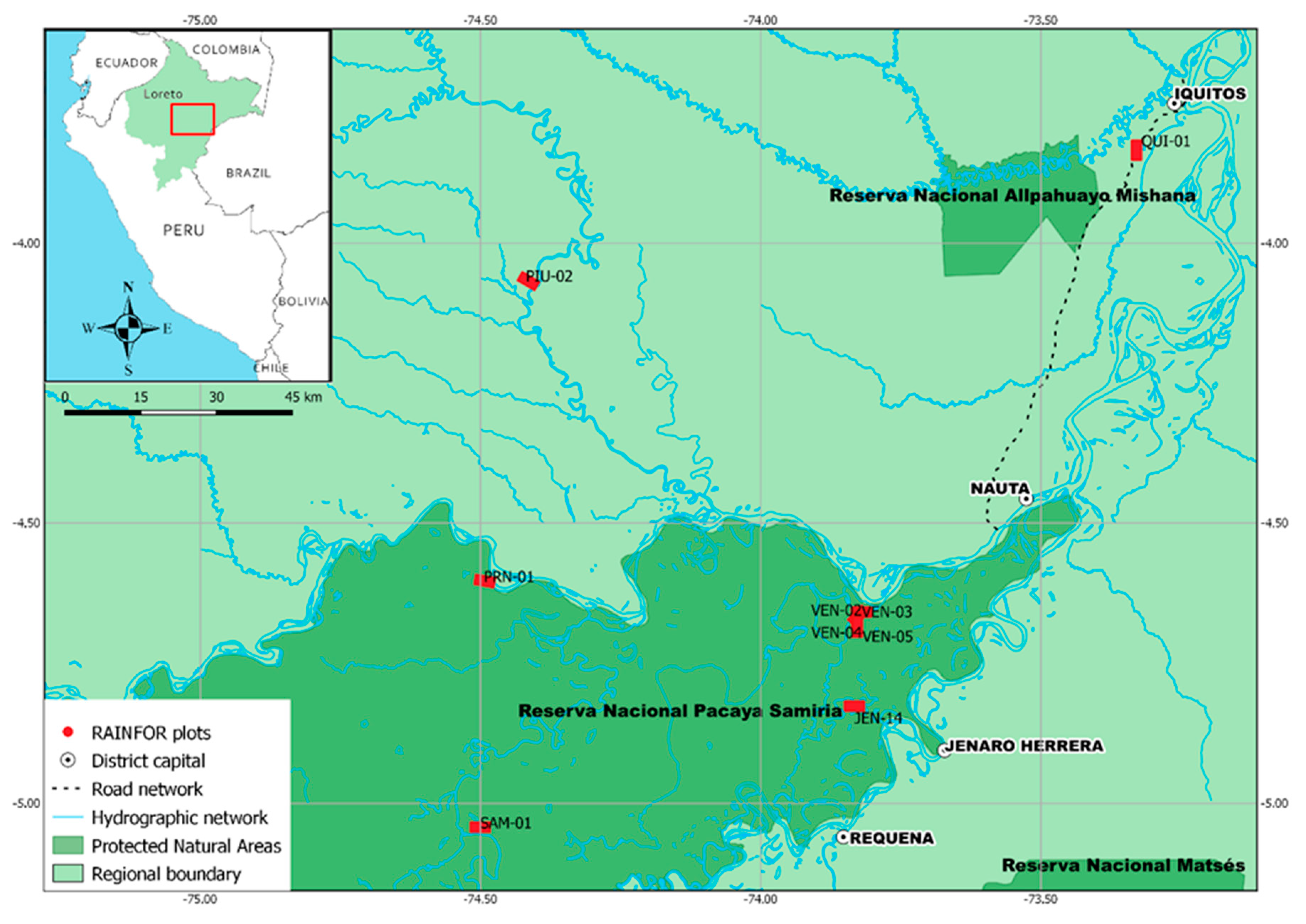
2.1. Study Area

We surveyed ten 0.5 ha permanent forest plots (50 m × 100 m) that were already established in palm swamps dominated by Mauritia flexuosa, locally known as “aguajales”. Plots were established inside protected natural areas and in forests managed by local communities in the region of Loreto, in northeastern Peru (Figure 1). Each plot contains different densities of palm trees. The plots belong to the Amazon Forest Inventory Network (RAINFOR) and were established using a standard protocol [44]. Plot data are managed using the ForestPlots.net online database [45,46].

2.2. Data Collection

Within each permanent plot, for each tree, the relative location within the plot, species and diameter at breast height (DBH) were recorded. The height of all the palm trees and the height of 10 random trees per diameter class were measured in the plot following the RAINFOR protocol. Information of the plots is summarized in Table 1. The geographic location of the plots and the location of the palm trees were recorded with the handheld GPS Trimble Geo7X and the dual-frequency GNSS Trimble Tornado antenna, with an average error of approximately 5 m.
The whole area of each plot was surveyed using a DJI Phantom 4 Pro (PH4 Pro) UAV from October to December 2017. The PH4 Pro is a rotary-wing aircraft with four propellers (quadcopter). It has 30 min of endurance when the payload is lower than 200 g and 12 min endurance at 400 g. The ground control station and the UAV are radio-linked at 2.4 GHz frequency. Users can control the UAV in either manual or automatic mode via a remote control connected to a tablet. The PH4 Pro consists of a GNSS (GPS + GLONASS), compass, vision system and a 20 megapixel (MP) 1” CMOS RGB camera attached to the bottom with a gimbal. The camera can record high-resolution images or high-definition videos (4K) and provides a real-time connection between the camera and the tablet [47].
The missions were performed at 60 and 90 m above ground level (AGL). The forward overlap was 88% and the side overlap was 83%. Mission details are listed in Table A1.

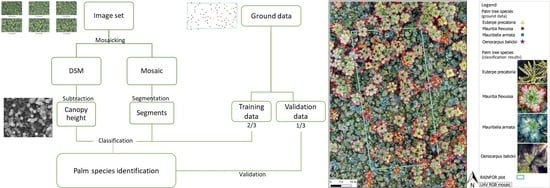
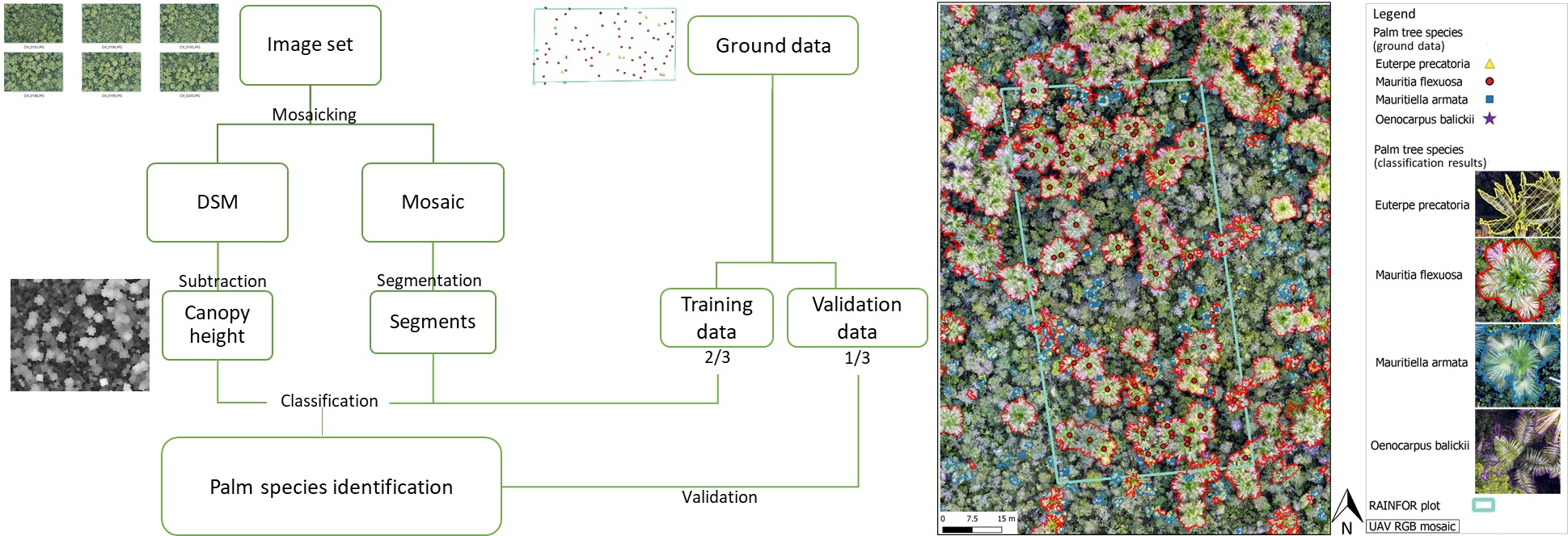
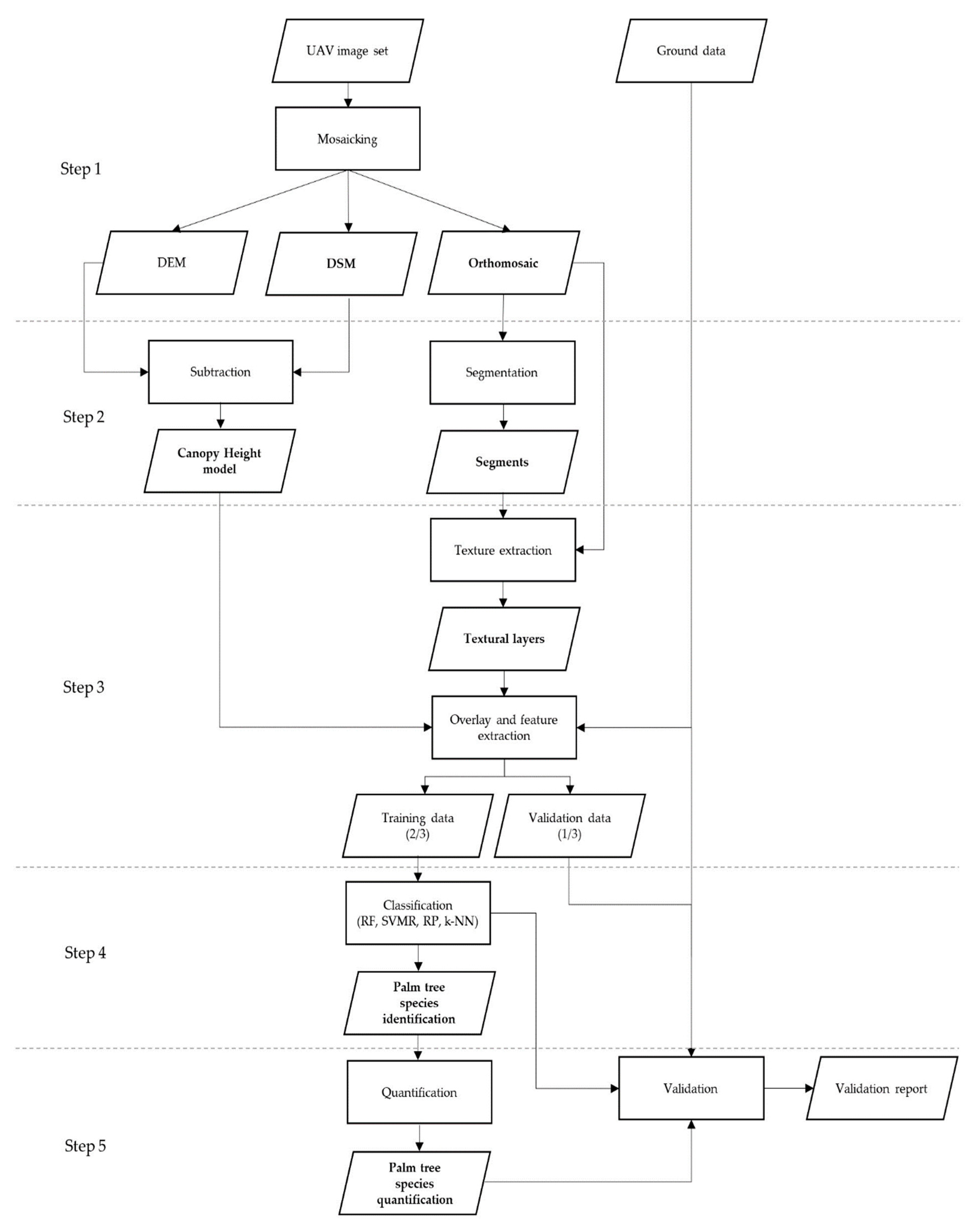
2.3. Data Processing

The UAV image processing comprised the following 5 steps: (1) mosaicking, (2) segmentation of the mosaic, (3) training samples preparation, (4) classification, and (5) palm tree quantification. Figure 2 shows the workflow. The mosaicking (Step 1) was carried out using the commercial software program Pix4D mapper [48] in a PC of 3.5 GHz 14-core with 128 Gb of RAM and an NVIDIA Quadro M4000 graphics processing unit (GPU). The rest of the steps were performed using the open-source software R v. 3.4.4 [49] in a laptop of 2.6 GHz quad-core with 16 GB of RAM and an NVIDIA Quadro M1000M graphic card. All the scripts generated in R, are available on the Github repository (https://github.com/xime377/UAV-classification). To speed up the testing process, the HPC Manati cluster was used. It has a coordinator node (Intel Xeon E5-2680 v4 2.40Ghz of 56 cores with 64 GB of RAM) and 9 processing nodes (Intel Xeon E5-2680 v4 2.40Ghz of 28 cores with 64 GB of RAM per node), 6 of these nodes have an NVIDIA Tesla K80 graphic card.
Pix4D mapper uses the Structure from Motion (SfM) algorithm in combination with dense image matching to generate a digital surface model (DSM) and the orthomosaic [50,51]. Since vegetation is difficult to reconstruct due to its complex 3D structure (leaves, branches), data from different UAV missions were combined and different parameters were tested to obtain orthomosaics with as few artifacts as possible. Forty-nine orthomosaics were obtained in total, having on average five mosaics per permanent plot. For further analyses, only one mosaic per plot was selected, visually selecting the one that showed the least artifacts. In some cases, the orthomosaic was acquired in one mission, in other cases, the pictures from different flights over the same plot were combined. The characteristics of the ten selected orthomosaics are presented in Table 2 and some mosaics are shown in Figure 3.
In Pix4D mapper, the process is divided into 3 tasks. First, the initial processing aligns the images and selects key points from visual similarities between the overlapping images acquired with the RGB camera. The full keypoint image scale was selected and the automatic rematch was enabled. Second, a dense point cloud was generated using the multiscale option, selecting the 1/4 and 1/8 of the full image, and the optimal point density. Third, the DSM, the digital terrain model (DTM) and the mosaic were produced using the inverse distance weight (IDW) method and a sharp smoothing filter.
The segmentation (step 2 of the workflow) was performed in the software program R and GRASS GIS 7.2.2. The R package rgrass7 [52] allows the implementation of GRASS GIS functions in R and facilitates the data exchange between the two software packages. The function i.segment [31] with the region growing and merging algorithm was used to group similar pixels into unique segments. This segmentation algorithm sequentially examines all the current segments in the orthomosaic, merging neighboring segments if they are similar or close according to the distance formula.
Two parameters are required to set the size of the segments: a threshold value and a minimum segment size. The threshold value ranges from 0 to 1, lower threshold values would allow only identical valued pixels to merge, while higher values would allow the merging of close pixels even if they are not similar. The minsize parameter sets the minimum number of pixels in a segment, merging small segments with a similar neighbor. At higher spatial resolutions, it is recommended to have a higher minimum segment size, in order to have larger and fewer segments per orthomosaic, that captures at least one palm leaf per segment. Since the segmentation is based on the number of pixels, and the orthomosaics generated had a very high resolution (1.22–2.09 cm), the orthomosaics were re-scaled to a pixel size of 5 cm, keeping enough details of the palm trees and reducing the computation time. In general, with smaller pixel sizes, there will be more segments because the orthomosaic contains more details.
Different combinations of these parameters were tested visually in order to obtain segments that captured the shape of palm tree leaves (Figure 4). Overall, we found that mosaics with 5 cm pixel size, a minimum size of grouping pixels was 50, and a similarity threshold of 0.05 best delineated the palm leaves.
The training sample preparation (Step 3) consisted of combining the ground data with the UAV data. The ground data comprised the palm tree locations recorded with the GPS and the Forestplots database. These data were linked, obtaining a shapefile with the palm tree tag, species name, and the RAINFOR measurements.
The UAV data consisted of the RGB mosaic, the canopy height model (CH), the segmentation output from Step 2 (a vector and a raster layer per mosaic) and the textural layers.
The shapefile layer with the ground data was overlaid on the RGB mosaic using the open-source software Quantum GIS (QGIS) to check if the location points corresponded to the palm tree crowns in the mosaic. Misaligned reference palm trees were manually aligned with the crowns in the mosaic based on the relative coordinates provided in the Forestplots database or not considered in the classification if the corresponding palm tree was not clearly identified in the mosaic. The details of the palm tree species considered for the classification are shown in Figure A1. In order to constrain the classification for the identification of palm tree species, some ground data of soil, water, and other trees were included as extra classes to avoid that the classifiers would identify them as palm trees.
The canopy height (CH) model was obtained using the package raster [53] in R. The UAV DTM was subtracted to the DSM to generate the CH layer. The textural characteristics of each segment of the orthomosaic were calculated in R, integrated with GRASS GIS 7.2.2. Table 3 gives a description of the features obtained during this step.
The textural layers and the CH were stacked and overlaid with the shapefile containing the ground data, assigning the values to the corresponding training point. The ground truth points were split into training (2/3) and validation (1/3) dataset.
The classification (Step 4) was performed in R, using the CARET package [54], short for Classification and REgression Training. Four non-parametric decision tree algorithms were tested: (1) Kernel Nearest Neighbor (k-NN), (2) Recursive Partitioning (RP), (3) Random Forest (RF) and (4) Support Vector Machine Radial (SVMR). The default parameters of the software were used in the classifiers.
The k-NN is commonly used for single tree detection in temperate forests [12,39]. It uses the Euclidean distance from the observation to be classified to the nearest training sample observation and assigns it to that class [39,55]. The RP creates a decision tree that splits the observations several times into homogeneous groups based on several dichotomous independent variables. The process is recursive because each observation set is split an indefinite number of times until the splitting process terminates after a particular stopping criterion is reached [55]. The RF is one of the most frequently used classifiers in forest remote sensing of forests because it provides accurate results and it is less sensitive to overfitting compared to other decision trees [12,37]. It is an ensemble decision tree classifier that uses bootstrap aggregated sampling (bagging) to construct many individual decision trees, from which a final class assignment is determined [36]. The SVMR is widely used when working with tree species classification because it is robust to noise and high-dimensional data, comparably few training data is needed, and it splits the data using a non-linear approach [12,37], suitable when working with complex canopy vegetation.
To evaluate the algorithms, an ANOVA test and the post-hoc Tukey honest significant difference test were conducted.
The general performance of the different models in the classification was evaluated with the overall accuracy and the Cohen’s kappa coefficient.
The overall accuracy (OA) is the total number of correctly classified segments (true positives, tp), divided by the total number of samples (Nc):
O A = c l a s s i t p N c ,
where i is the number of classes.
The Cohen’s Kappa coefficient (κ) is a statistic that measures the agreement of prediction with the true class. It takes into account the possibility of the agreement occurring by chance (expected accuracy, EA).
k = O A E A 1 E A ,
E A = c l a s s i t p N c × f p N c ,
where fp is the number of segments predicted as positive that were actually negative (false positives).
The species identification assessment consisted of the producer and user accuracy, and the corresponding confusion matrices. The producer’s accuracy (PA) is derived by dividing the number of correctly classified segments per class (tp) by the total number of segments corresponding to the ground truth of that class:
P A c l a s s = t p c l a s s N g r o u n d   t r u t h   c l a s s ,
The user’s accuracy (UA) is the number of correctly classified segments (tp) in a class divided by the total number of segments that were classified in that class:
U A c l a s s = t p c l a s s N c l a s s i f i e d ,
After the classification step was conducted using all the predictors, the variable importance of the random forest models was analyzed to identify the layers that have the most predictive power in the classification per plot (feature selection). The variable importance was obtained from each plot model using the CARET package [54] in R. The layers that had repeatedly higher importance among all the plots were selected as the ones that contributed the most to palm identification.
The palm tree species quantification (Step 5) was performed in R, using the packages raster [53] and simple features [56]. This Step was mainly needed since the study area is a tropical forest dominated by Mauritia flexuosa palms and, in most cases, they were too close to each other, having many crowns in only one object. For this reason, this Step was conducted to split the crowns mask and obtain single crowns to be counted. This Step is not needed in areas with a lower density of palm species. The splitting process consisted of intersecting the five height classes from the K-means unsupervised classification of the canopy height model, with the classification crown mask. Finally, a table with the count of individuals per palm tree species was generated.
The accuracy of the palm tree quantification for each plot was determined by comparing the palm trees that were recorded during the ground data survey, and also the visible palms on the orthomosaics, with the palm trees detected by the classification algorithm. The precision, recall and F1 score were calculated per plot.
The precision is the number of polygons correctly classified (tp) as the corresponding palm species divided by the total number of polygons (Nq) generated in the quantification step:
P r e c i s i o n = t p N q ,
The recall is the number of polygons correctly classified (tp) as the corresponding palm species divided by the total number of ground truth data. In this case, we calculated the recall with the number of visible palms in the mosaic (Recallvisible) and the recall with the number of all the palm trees measured on the ground (Recallground):
R e c a l l v i s i b l e = t p N o .   o f   v i s i b l e   p a l m s   i n   t h e   m o s a i c ,
R e c a l l g r o u n d = t p N o .   o f   p a l m   t r e e s 10 c m   d b h   o n   t h e   g r o u n d ,
The F1 score is the harmonic mean of recall and precision and thus it expresses the balance between recall and precision:
F 1   s c o r e = 2 × p r e c i s i o n   × r e c a l l p r e c i s i o n + r e c a l l ,
The F1 score was calculated for both cases: using the Recallvisible and the Recallground. This evaluation index was used in this case instead of the overall accuracy because, unlike in the classification step where the number of segments per class was similar, the abundance of Mauritia flexuosa in most of the plots was higher than the abundance of the other palm species.

3. Results

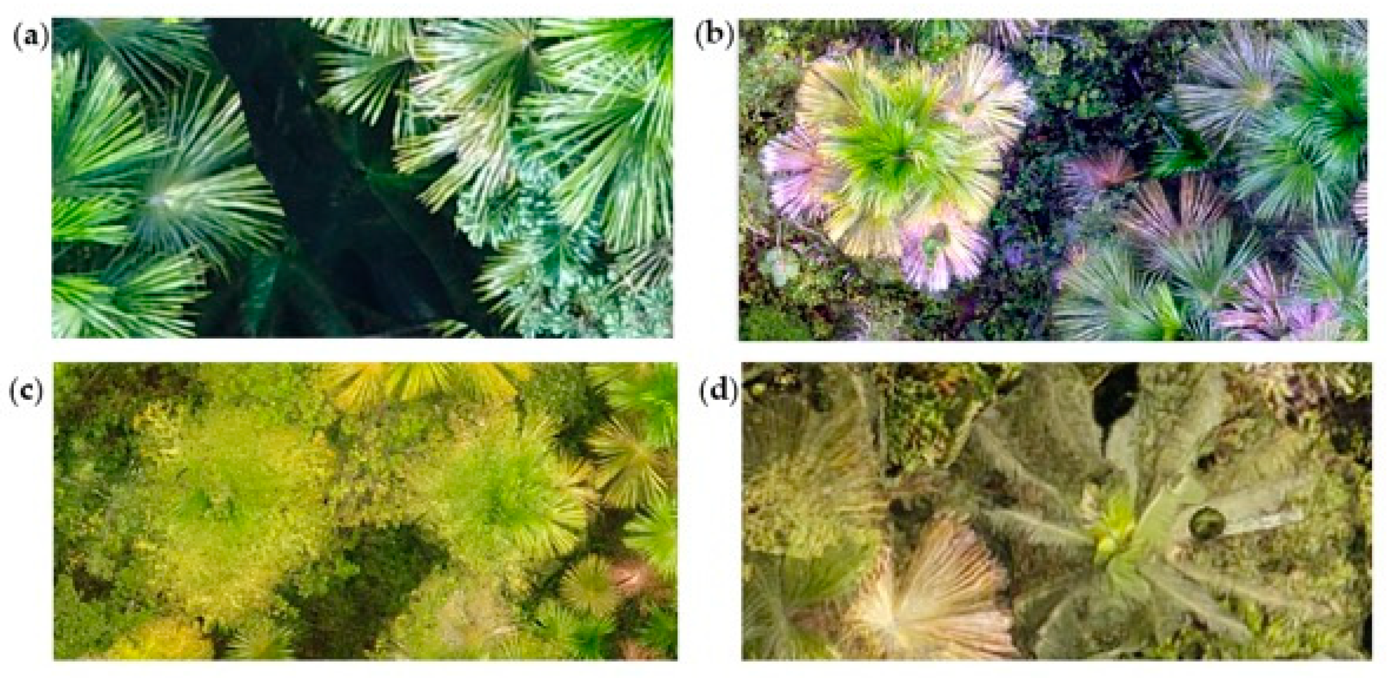
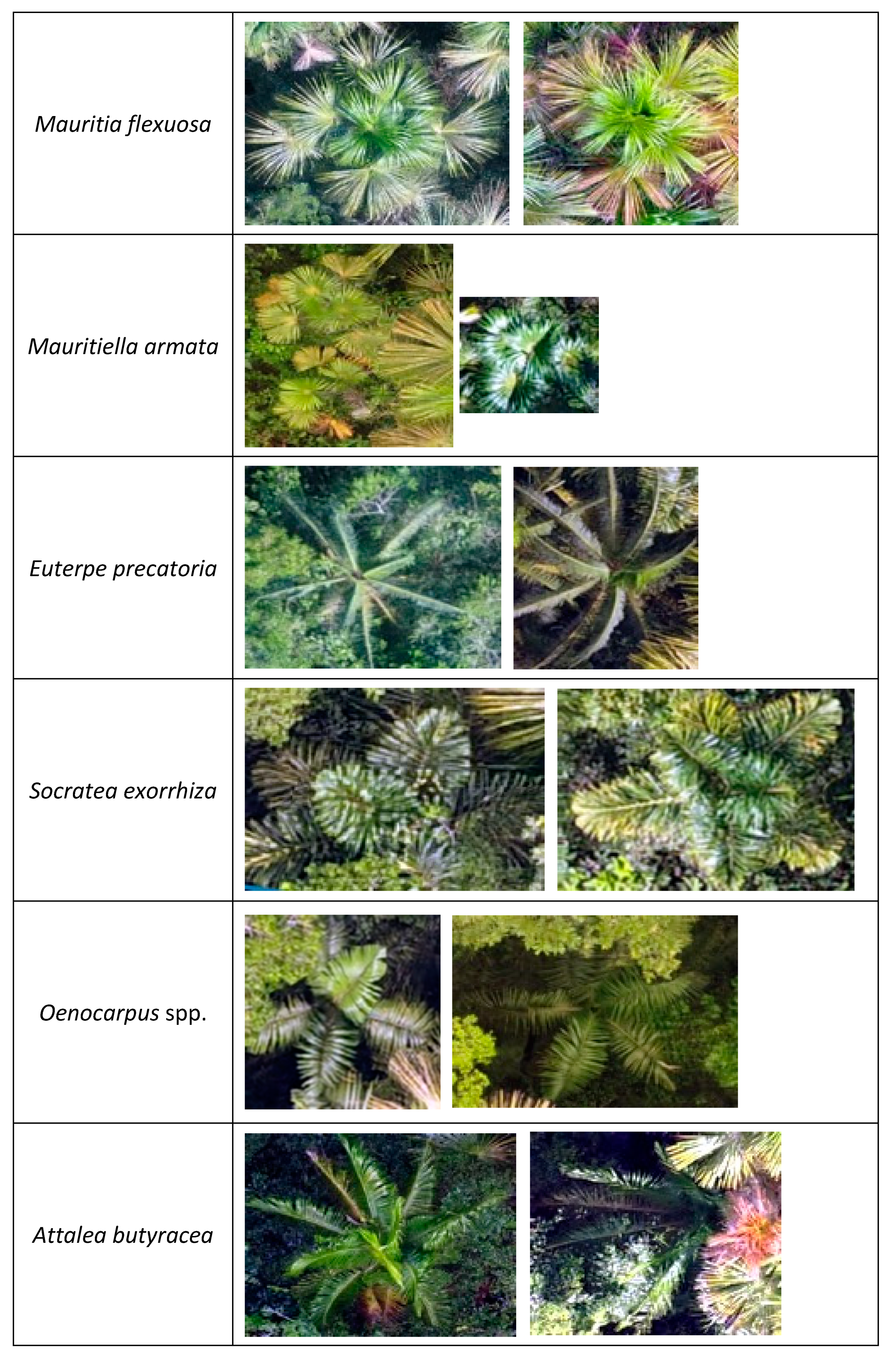
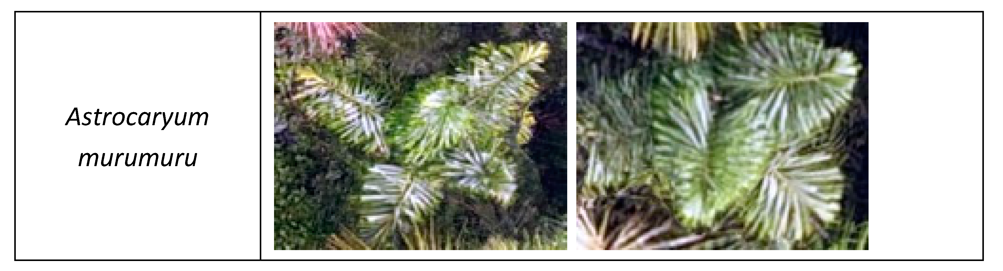
3.1. Palm Species Identification

The palm tree species identification was performed using different classifiers. The Random Forest (RF) algorithm was the one with the highest overall accuracy (85% in average) and kappa coefficient (0.82 in average), closely followed by the Support Vector Machine Radial (SVMR) with 85% overall accuracy and Cohen’s Kappa coefficient of 0.81 on average. There was no statistically significant difference between the results obtained from RF and SVMR, but the results of those algorithms were significantly higher than those obtained from k-NN and Recursive Partitioning (p < 0.001, 95%). Table A2 presents the evaluation of the different methods used.
When examining the detection success per palm tree species, the identification of M. flexuosa was the most accurate since it was the dominant species in all plots. There was a general overestimation of the non-canopy dominant species (Astrocaryum murumuru and Oenocarpus spp.) and species with a small amount of training data (Socratea exorrhiza, Euterpe precatoria, and Attalea butyracea). The species that were not canopy dominant appeared more often with shadows, lacking enough good quality training data, and were misclassified as dark parts of trees or artifacts. In most of the cases, the classification was able to predict correctly Mauritia flexuosa, Mauritiella armata, and Euterpe precatoria even outside of the plots. Since there was no training/validation data for those areas, this was only verified visually. One of these cases is VEN-05 plot. Figure 5 shows the classification results of VEN-05 and PRN-01 RAINFOR plots.
On the other hand, plots with palm tree species with a very different crown shape, tend to obtain higher accuracy values. This can be seen when comparing QUI-01 and PIU-02, two plots with the same number of palm species and similar M. flexuosa abundance (Table 1). QUI-01 had a lower classification accuracy due to the presence of Mauritiella armata and less palm visibility (κ = 0.72), while PIU-02 composed just of M. flexuosa and E. precatoria, had a Cohen’s Kappa coefficient of 0.86.
More complexity is added when the plots have more palm tree species, as some of the crowns of the species look similar and there is only a small amount of training data for the non-dominant species. This is the case of PRN-01, where S. exorrhiza was classified as M. flexuosa or A. murumuru and viceversa; and Mauritia flexuosa and Mauritella armata were also misclassified (Table 4).

3.2. Feature Selection

Five layers contributed the most to palm species identification: (1) the canopy height model, (2) compactness of the segments, (3) median of the green band values per segment, (4) mean of the sum of variance of the green band values per segment, and (5) the mean entropy of the red band values per segment. The impact on the species discrimination is shown in Figure 6; the accuracy assessment using these 5 predictors is shown in Table A3.

3.3. Palm Tree Species Quantification

The palm species quantification performed better in plots where the palm density was lower or the palms that were close to each other had different heights. The results of the quantification step using the output from the random forest classification were compared with the number of visible palms in the UAV orthomosaic obtaining on average a Recall of 71.6% and an F1 score of 0.65, and with all the geolocated palms in the RAINFOR plot (average Recall = 51.4%, F1 score = 0.65). The accuracy assessment per RAINFOR plot can be seen in Table A4. Figure 7 shows the comparison of the results obtained for the Mauritia flexuosa and Mauritiella armata species with the number of visible palms in the UAV orthomosaic (Figure 7a,b) and with all the geolocated palms in the RAINFOR plot (Figure 7c,d).
The number of palm tree stems captured by the UAV is lower than the ground data, capturing on average 69.8% of the palms present in the forest plots. This value strongly depends on the canopy density of the plot, varying from 58% in dense palm swamps, to 86% in less dense areas (Table A5). This occurs because the RGB camera only registers the top of the canopy. In Figure 7c,d, this “underestimation” of the understory palms can be seen. The points with similar values in the comparison with visible UAV palms (Figure 7a,b) and in the comparison with all the field measurements (Figure 7c,d), correspond to the plots with higher palm visibility. The quantification of these palms is more successful if there is higher palm visibility and if the palm species composition is more diverse or they are not too close to each other.

4. Discussion

This study is one of the first attempts to detect and quantify native palm species in a complex forest such as Amazonia. Most of the previous studies that allow detection and quantification using a segmentation step before conducting the classification have been performed either in plantations [28,57] or in open forests [32], areas where the studied features are easily discriminated due to the high contrast of them with the background. In all these studies, the presence of bare soil or very little presence of small plants in the background makes easier the detection and quantification process. In plantations, the systematic arrangement of the plants facilitates the detection more notably. The workflow here managed to identify and quantify the palm tree species from RGB UAV imagery in a tropical rainforest, where almost the whole mosaic consists of green vegetation. The approach was successful in detecting palm trees due to their distinctive crowns in the rainforest [40]. The assessment of the method using ten permanent plots with 1170 reference palm trees demonstrated that small UAVs with RGB cameras are useful for mapping this aspect of tree biodiversity in tropical forests.

4.1. Palm Tree Identification and Classification Results

The workflow developed here allows a semi-automatic classification using open-source software to detect different palm species in a complex environment. The segmentation process is one of the key steps for the correct identification of the palm species and it speeds up the processing times as mentioned in previous research [29]. It is recommended to try to get larger segments with higher similarity values to delineate the object of study properly. Since we are working with high-resolution images, it is important to consider that the smaller the pixel size, the more pixels per mosaic and thus more segments obtained [31]. This will influence the computational requirements and processing times.
In general, the accuracy of the classification was determined by plot species composition and vegetation density (expressed here as the palm visibility in the UAV mosaic). This is the case of QUI-01, VEN-04 and VEN-05, where the palm tree composition was characterized by Mauritia flexuosa and Mauritiella. armata. The main difference between these species is the size of leaves when looking from above (Figure A1), and thus, the misclassification occurred in both directions (Table 4). VEN-05 had a higher classification accuracy (κ = 0.84) due to the lower stem density and higher palm tree visibility in the plot, with more space between palm trees (Figure 5a).
Considering that the workflow uses a relatively small amount of training data since one palm tree could have more than one segment, it is important to have good-quality training data. This is related to data acquisition: the mosaics should have enough quality to be able to extract features from them, and the mosaic should contain enough features to train and validate the model. This can be seen in the lower classification accuracy in plots where there was a lack of good-quality training data, either due to illumination conditions as the case of E. precatoria, or where there were not enough palm trees per species as the case of A. butyracea (Table 4). This methodology would also not be suitable to study understory palm tree species since the RGB UAV imagery only captures the top of the canopy.
Since there were no radiometric corrections performed in the UAV images, illumination conditions and the solar elevation angle influenced the results of the classification. Missions conducted when there was a clear sky tended to have saturated images (like in the mosaics of PRN-01 and SAM-01), resulting in M. flexuosa and E. precatoria palms with white leaves. This caused some trees to be classified as M. flexuosa or vice versa when there were white branches similar to the border of the M. flexuosa palm leaves. In the plots with the presence of E. precatoria, the overestimation of the species occurred due to the similarity of the long leaves with some bright tree branches. Missions conducted when the solar elevation angle was low (<30°, such as in the mosaic of VEN-02 plot, mission details on Table A1), provided images with more shadows, having similar misclassification issues as mentioned before (trees classified as palms and viceversa). One way of reducing the illumination effect could be the use of ratios between the different color bands as a preprocessing step, as the normalized ratio between the red and green bands of the RGB mosaic [21].
As mentioned in Section 3.1, the accuracy of the classification is lower when the shape of the palm tree leaves are similar. During this study, some plots contained two species that look similar from above: M. armata and M. flexuosa. M. armata has smaller costapalmate leaves with a circular outline. The stems are clustered with short, stout, conical spines (usually not seen from the top of the canopy). M. flexuosa has costapalmate leaves with a circular outline deeply split in half, and each half is split into numerous leaflets and the tips of the leaflets tend to spread in different planes. Looking from the ground, it can be seen that this palm has a solitary stem [41]. In this classification method, the Canopy height model helped to discriminate them because M. flexuosa reaches greater heights. In addition, the different size of the leaves was reflected in the compactness of the segments, and the fact that the leaves have a different arrangement leads to different values of entropy for the two species. However, differentiating other groups of similar species may be challenging [58]. For example, Cecropia latiloba (a tree with somewhat similar leaf characteristics as M. armata in a UAV image) in some plots tends to be predicted as M. armata. A similar case could occur if the palms Socratea exorrhiza and Iriartea deltoidea are found in the same image, as from above, the crown shapes look similar [40]. To overcome this challenge, other types of technologies like hyperspectral imagery or Lidar techniques could be used in the future [58,59].
In terms of processing times, the most time-consuming operations were the texture extraction and value extraction from the raster. These tasks strongly depend on the size of the mosaic. They can be sped up by working only with the five suggested layers as mentioned in Section 3.2 or splitting the mosaic in tiles that are subsequently merged. Table A6 shows the computational time consumed by each step of the workflow.

4.2. Feature Selection

The canopy height model (CH) was the layer that contributed the most to the classification. It helped to discriminate lower areas like the soil and water, but it also contributed to discriminate canopy dominant species such as M. flexuosa and lower canopy species like Oenocarpus spp. The compactness layer, since it is related to the size and shape of the segments, helped to identify larger segments as tree crowns, elongated segments as E. precatoria and compact star-shaped segments as Oenocarpus spp. This layer is quite important for the robustness of the model because it helps to discriminate species by its shape when color layers do not provide much information due to changes in illumination conditions and a lack of radiometric corrections. A clear example can be seen in Figure 6, in the compactness of VEN-02 (blue frame), where some of the training samples were shaded but the segmentation step managed to capture the shape of these palms.
The median values of the green band contributed to discriminate Mauritiella armata and Mauritia flexuosa from the rest of palm species due to the intense green leaves, and in some cases, helped to distinguish Mauritiella armata (paler green) from M. flexuosa.
The sum of variance of the green band and the mean entropy values of the red band provided information about the complexity within the mosaic. Palms with leaves spread in different planes tend to have higher entropy values. These layers contributed to discriminate A. murumuru from E. precatoria (it has leaves in one plane) and M. flexuosa from S. exorrhiza (plumose appearance).
Even though different object parameters were calculated, only compactness was chosen as the layer contributing the most to the model (Section 3.2). This is because the different parameters are often correlated: for instance, both compactness and the fractal dimension (fd) are derived from the length of a segment. Compactness and fd have a negative correlation because while compactness indicates homogeneity, fractal dimension indicates heterogeneity [35]. Regarding the textural variables, the entropy and sum of variance work as an indication of the complexity within the mosaic [35], contributing to the discrimination of different palm species due to their different leaf arrangements. In this sense, the fact that only a few layers contribute to the classification accuracy makes the process easy to understand and to be replicated.
However, in most of the cases M. flexuosa, Mauritiella armata, A. butyracea, and S. exorrhiza were hard to differentiate: the first two, due to the similarity in the leave shape, and the latter due to the lack of enough good quality training data (images with strong shadows are prone to misclassification).

4.3. Palm Tree Quantification and Validation Data

The palm tree quantification works well for areas with low palm tree density or areas with a high diversity of species since the chances of finding palms close to each other in one area are lower. When the palm species were too close to each other and they had similar heights, obtaining individual crowns was not possible and there was an underestimation of the quantification. In other cases, the splitting step caused an overestimation of the palms due to the variation in height within a single crown (higher heights in the center of the crownshaft and lower heights around it).
The number of palms captured by the UAV imagery strongly depends on the canopy density, with more visible palms in less dense areas. This method is suitable for counting canopy dominant species since understory species could appear in the UAV mosaics, but they would be partially covered by the leaves of other species and separate parts of a visible crown may be counted as different individuals. This part of the workflow was designed as a quick alternative to split crowns that are grouped as one object after the classification step.
It is important to mention that a small part of the overestimation of palms in Figure 7a,b is also due to the detection of palms with a dbh lower than 10 cm, which are not geolocated, nor considered in the RAINFOR protocol. In plots with 57%–58% of palm visibility, there were no differences in the counting; however, in plots with 67% or higher palm visibility, palms with dbh lower than 10cm start appearing in the mosaics. Considering that the number of palms measured on the ground was 1676, the number of stems that were not georeferenced was less than 1%.

4.4. Considerations for Image Acquisition

Image capture needs to deal with variation in the illumination conditions due to cloudiness, blurry images or moving objects due to winds. These issues need to be considered for the mosaicking Step, especially if data from different missions are combined. Regarding the illumination conditions, since the fieldwork was conducted in the tropics, the suitable flying hours do not vary much throughout the year; however, variation during the day is crucial. The solar elevation angle influenced the results of the mosaicking and classification due to its influence on the presence of shadows (Figure 8a). As a result, it is recommended to fly when the solar elevation angle is higher than 30° (usually from 8:00–15:00 hours). Clouds also contribute to the presence of shadows, especially when there are the “popcorn” clouds. Overcast conditions provided more homogeneous mosaics, whereas clear sky conditions lead to saturated images. The result of combining missions with different illumination conditions (either different flying hours or presence of clouds) without a prior image normalization is a patchy mosaic (Figure 8b). For the aim of this research, radiometric calibration is not crucial since the classification is mainly based on geometrical patterns, compactness of the segments and textural information. However, the results could be improved if some brightness/shadow corrections could be conducted when the images are too dark to recognize similar pixels. Otherwise, those dark pixels will be recognized as ground by the SfM software and the segmentation step.
When combining missions when there was wind, the resulting mosaics are blurred or, in some cases, stitching was not even possible. Figure 8c shows part of a mosaic generated from one mission with strong wind, in which the palm trees are only partially visible. Even though the PH4 Pro is water-resistant [47], the pictures captured during rain events can also contain droplets of water. Even if the SfM software is able to generate a mosaic, some blurry areas may occur, or the whole mosaic may be blurry (Figure 8d), which prohibits proper segmentation and leads to poor classification results. For this reason, it is not recommended to acquire the images under poor weather conditions, like the ones described in this section.
Another important consideration is the flying height: most of the mission planning software takes into consideration the flying height above ground level (AGL), but the level of detail in a forest depends on the above canopy level (ACL). For this reason, it is necessary to know in advance the average canopy height and the maximum height of the trees. For this study, the best mosaics were obtained from the missions flying 60 m above the canopy, and, since the level of detail was extremely high, it may be possible to fly even higher (for instance 120 m AGL) in order to reduce some variation in leaves and to cover more area. With a spatial resolution of 5 cm, the level of detail was sufficient to distinguish the palm species.

4.5. Further Implications

The workflow developed here could also be applied to a different study object if it has a distinctive texture or shape and if the input parameters are tuned to do so. Moreover, this methodology could also be applied to high-resolution satellite imagery if the palm crowns are clearly visible. For example, the WorldView-3 satellite imagery (spatial resolution of 0.3 meters) can easily display the crowns of Mauritia flexuosa since the crown diameter of this palm species is on average 8 meters.
The segmentation step of this workflow could be helpful when working with deep learning and semantic classification. It could help to prepare the training data instead of delineating the features manually or using commercial software as was the case in [28] who used segments from UAV imagery for training a CNN to delineate citrus trees.
From an ecological point of view, small UAVs with only RGB cameras provide useful information in larger areas than the usually covered just by doing conventional ground-based surveys. Flying over a 0.5 ha plot took around 20 min including the assembling of the equipment and the UAV products can be used to derive different ecological indicators. The products obtained from the SfM software were the RGB mosaic, the digital surface model (DSM), and the digital terrain model (DTM). From the RGB mosaic, it is possible to visualize the emergent species and determine some illumination characteristics. If the mosaic is further processed as in this study, the combination with ground data makes possible the quantification of the canopy dominance per palm species by calculating the area of each of the species mask obtained from the classification. The gap area can also be quantified by calculating the area of the mask generated for the classes “soil” and “water”. The canopy height model can be derived from the DSM as was described in Section 2 and it could provide some information about the structure of the canopy.

5. Conclusions

A complete method for identification and quantification of the abundance of economically important palms using RGB UAV imagery in the rainforest was generated using open-source software. The process comprises mosaicking, segmentation of the mosaic, training samples preparation, classification, and palm tree quantification. Five descriptors were selected as the most useful for species discrimination, integrating canopy height with shape and textural characteristics. The workflow was tested in ten 0.5 ha permanent plots, using 1170 reference palm trees, providing good classification results. The method is suitable for areas where the palm density is medium to low, and the palms are not too close to each other. The use of small UAVs with RGB cameras, in combination with field data, has the potential to provide estimates of resource availability at relevant scales for tropical forest management, especially where cloud cover limits the use of satellite imagery, and the large areas and accessibility restrict ground-based surveys.

Author Contributions

X.T.C., E.N.H.C., and T.R.B. conceived and designed the methodology; X.T.C., L.F., and G.F. collected and processed the ground data; X.T.C., L.F., and R.C. processed the UAV data; X.T.C., H.B., T.R.B., and M.H. conducted the formal analysis. All authors contributed to drafts and gave final approval for publication. All authors have read and agreed to the published version of the manuscript.

Funding

The fieldwork campaign for this research was funded by the Gordon and Betty Moore Foundation through the grant ‘Monitoring Protected Areas in Peru to Increase Forest Resilience to Climate Change’ (MonANPeru) led by T.R.B. IIAP contributed to the cost of equipment acquisition. Funding to X.T. from the Russel E. Train Education for Nature Program (EFN) from WWF, Wageningen University and the FONDECYT grant agreement 219-2018 contributed to the analysis and completion of the manuscript.

Acknowledgments

This study was supported by the IIAP (BIOINFO and PROBOSQUES research programmes), with special thanks to Americo Sanchez and Dennis Del Castillo for their assistance. We would like to thank Jhon Del Aguila, Julio Irarica, Hugo Vásques and Rider Flores for their help while conducting fieldwork.

Conflicts of Interest

The authors declare no conflict of interest.

Appendix A

Table A1. Information of the UAV missions performed.
PlotMissionFlying Height AGL (m)Flying Height ACL (m)Area Covered (ha)No. Total ImagesAcquisition DateCloud CoverSolar Elevation (°)Wind Speed
JEN-14JEN-14_190701.002418-10-17overcast31.73calm
JEN-14JEN-14_250301.056618-10-17partly cloudy35.17calm
JEN-14JEN-14_390701.671918-10-17overcast54.12calm
JEN-14JEN-14_490701.052415-12-17partly cloudy56.97calm
JEN-14JEN-14_565451.336015-12-17partly cloudy57.76> 3 m/s
PIU-02PIU-02_190703.639526-11-17clear sky49.59calm
PIU-02PIU-02_265453.229526-11-17clear sky54.57calm
PRN-01PRN-01_190703.848620-11-17clear sky59.70medium
PRN-01PRN-01_260402.039220-11-17partly cloudy65.16calm
QUI-01QUI-01_190703.359409-12-17partly cloudy56.84calm
QUI-01QUI-01_265452.608509-12-17clear sky66.36calm
SAM-01SAM-01_190701.233518-11-17clear sky51.20calm
SAM-01SAM-01_290701.123018-11-17clear sky55.88calm
SAM-01SAM-01_360401.126118-11-17clear sky56.97calm
VEN-01VEN-01_190700.842706-10-17partly cloudy85.39calm
VEN-01VEN-01_265450.985006-10-17partly cloudy86.86calm
VEN-02VEN-02_190700.694705-10-17clear sky29.87calm
VEN-02VEN-02_260400.698405-10-17clear sky27.88calm
VEN-02VEN-02_465451.764606-10-17clear sky40.76calm
VEN-03VEN-03_290700.794706-10-17partly cloudy52.56calm
VEN-03VEN-03_365450.797906-10-17partly cloudy55.30calm
VEN-04VEN-04_190700.914605-10-17clear sky81.38calm
VEN-04VEN-04_265450.816906-10-17partly cloudy41.86calm
VEN-05VEN-05_190701.296405-10-17partly cloudy46.76calm
VEN-05VEN-05_265450.938305-10-17partly cloudy53.23calm

Appendix B

Figure A1. Snippets from the orthomosaics that show the palm tree species used for the study.
Remotesensing 12 00009 g0a1aRemotesensing 12 00009 g0a1b

Appendix C

Evaluation of the different classification methods used
Table A2. Classification accuracies of the tested classification methods with all the predictors.
Plotk-NNRPRFSVMR
Acc.ΚAcc.κAcc.ΚAcc.κ
JEN-140.860.830.820.780.900.880.890.87
PIU-020.820.780.820.770.890.860.890.86
PRN-010.590.540.650.600.850.830.890.88
QUI-010.640.530.690.590.790.720.720.63
SAM-010.710.650.710.650.860.830.890.87
VEN-010.610.540.680.620.840.810.850.82
VEN-020.690.640.720.670.830.800.870.85
VEN-030.720.650.750.690.860.830.790.74
VEN-040.650.530.720.630.810.750.780.71
VEN-050.680.570.820.760.880.840.890.86
Mean0.700.620.740.680.850.820.850.81
Abbreviations: k-NN (k-Nearest Neighbors), RP (Recursive Partitioning), RF (Random Forest), SVMR (Support Vector Machine Radial).
Table A3. Classification accuracies of the tested classification methods with only the selected predictors (CH, compactness, median values of the Green band, mean entropy of the red band and the mean sum of variance of the green band).
Plotk-NNRPRFSVMR
Acc.κAcc.κAcc.κAcc.κ
JEN-140.690.610.830.790.850.810.850.83
PIU-020.650.570.760.700.770.710.770.71
PRN-010.550.500.580.530.780.750.780.75
QUI-010.550.410.700.600.730.640.730.64
SAM-010.610.520.680.600.880.850.820.77
VEN-010.500.400.670.610.770.720.770.72
VEN-020.530.450.660.600.710.660.710.66
VEN-030.630.530.740.670.790.720.790.74
VEN-040.610.470.770.700.770.690.770.69
VEN-050.570.420.750.670.780.700.780.70
Mean0.590.490.710.650.780.730.780.72
Abbreviations: k-NN (k-Nearest Neighbors), RP (Recursive Partitioning), RF (Random Forest), SVMR (Support Vector Machine Radial).

Appendix D

Table A4. Accuracy assessment of the quantification step per RAINFOR plot.
Evaluation indexJEN14PIU02PRN01QUI01SAM01VEN01VEN02VEN03VEN04VEN05
Number of correctly detected palm trees9558103965645112976678
Number of all the detected objects in the mosaic15292151143179134144111125111
Number of all the visible palm trees in the mosaic966013411910677154148171105
Number of all the palm trees with a DBH higher than 10 cm (Ground data)12876197204123132268196221123
Precision (%)62.5063.0468.2167.1331.2833.5877.7887.3952.8070.27
Recall with Visible palms in the mosaic (%)98.9696.6776.8780.6752.8358.4472.7365.5438.6074.29
Recall with Ground data (%)74.2276.3252.2847.0645.5334.0941.7949.4929.8663.41
F1 score with Visible palms in the mosaic0.770.760.720.730.390.430.750.750.450.72
F1 score with Ground data0.680.690.590.550.370.340.540.630.380.67

Appendix E

Table A5. Ground palm tree data per RAINFOR plot.
Species/PlotJEN14PIU02PRN01QUI01SAM01VEN01VEN02VEN03VEN04VEN05Total
A. murumuru00300000003
A. butyracea0000150000015
E. indet01000000001
E. precatoria3531113837500121
Indet indet05200000007
M. flexuosa124711098810471184180129801140
M. armata0014115003119243278
Oenocarpus spp.00600120009
S. exorrhiza1034032242000102
Total128821992041231322681962211231676

Appendix F

Table A6. Processing time consumed per step of the suggested workflow in a laptop with 16 GB of RAM and a Intel® Xeon® E-2156M CPU of 2.70GHz. The colored areas correspond to the time spent in one core of the HPC cluster with 64 GB of RAM and a Intel® Xeon® E5-2680 v4 CPU of 2.40GHz.
MissionMosaic Area (ha)SegmentationTexture ExtractionTraining SetClassificationQuantification
JEN-140.773 min27 min6 min12 min4 min
PIU-022.146 min50 min20 min24 min5 min
PRN-012.154 min32 min20 min18 min5 min
QUI-013.1313 min30 min10 min16 min6 min
SAM-010.995 min26 min47 min16 min1 min
VEN-011.454 min39 min10 min24 min1 min
VEN-021.327 min43 min1 h 20 min19 min5 min
VEN-031.359 min25 min6 min13 min12 min
VEN-041.043 min21 min43 min3 h 42 min1 min
VEN-052.3110 min34 min12 min14 min8 min

References

  1. Eiserhardt, W.L.; Svenning, J.C.; Kissling, W.D.; Balslev, H. Geographical ecology of the palms (Arecaceae): Determinants of diversity and distributions across spatial scales. Ann. Bot. 2011, 108, 1391–1416. [Google Scholar] [CrossRef] [PubMed] [Green Version]
  2. Couvreur, T.L.P.; Baker, W.J. Tropical rain forest evolution: Palms as a model group. BMC Biol. 2013, 11, 2–5. [Google Scholar] [CrossRef] [PubMed] [Green Version]
  3. Smith, N. Palms and People in the Amazon; Geobotany Studies; Springer International Publishing: Cham, Switzerland, 2015; ISBN 978-3-319-05508-4. [Google Scholar]
  4. Vormisto, J. Palms as rainforest resources: How evenly are they distributed in Peruvian Amazonia? Biodivers. Conserv. 2002, 11, 1025–1045. [Google Scholar] [CrossRef]
  5. Horn, C.M.; Vargas Paredes, V.H.; Gilmore, M.P.; Endress, B.A. Spatio-temporal patterns of Mauritia flexuosa fruit extraction in the Peruvian Amazon: Implications for conservation and sustainability. Appl. Geogr. 2018, 97, 98–108. [Google Scholar] [CrossRef]
  6. Roucoux, K.H.; Lawson, I.T.; Baker, T.R.; Del Castillo Torres, D.; Draper, F.C.; Lähteenoja, O.; Gilmore, M.P.; Honorio Coronado, E.N.; Kelly, T.J.; Mitchard, E.T.A.; et al. Threats to intact tropical peatlands and opportunities for their conservation. Conserv. Biol. 2017, 31, 1283–1292. [Google Scholar] [CrossRef] [Green Version]
  7. Draper, F.C.; Roucoux, K.H.; Lawson, I.T.; Mitchard, E.T.A.; Honorio Coronado, E.N.; Lähteenoja, O.; Torres Montenegro, L.; Valderrama Sandoval, E.; Zaráte, R.; Baker, T.R. The distribution and amount of carbon in the largest peatland complex in Amazonia. Environ. Res. Lett. 2014, 9, 124017. [Google Scholar] [CrossRef]
  8. Virapongse, A.; Endress, B.A.; Gilmore, M.P.; Horn, C.; Romulo, C. Ecology, livelihoods, and management of the Mauritia flexuosa palm in South America. Glob. Ecol. Conserv. 2017, 10, 70–92. [Google Scholar] [CrossRef]
  9. Nobre, C.A.; Sampaio, G.; Borma, L.S.; Castilla-Rubio, J.C.; Silva, J.S.; Cardoso, M. Land-use and climate change risks in the Amazon and the need of a novel sustainable development paradigm. Proc. Natl. Acad. Sci. USA 2016, 113, 10759–10768. [Google Scholar] [CrossRef] [Green Version]
  10. Monitoring of the Andean Amazon Project (MAAP). Deforestation Hotspots in the Peruvian Amazon, 2012–2014|MAAP—Monitoring of the Andean Amazon Project. Available online: http://maaproject.org/2018/hotspots-peru2017/ (accessed on 21 February 2018).
  11. Falen Horna, L.Y.; Honorio Coronado, E.N. Evaluación de las técnicas de aprovechamiento de frutos de aguaje (Mauritia flexuosa L.f.) en el distrito de Jenaro Herrera, Loreto, Perú. Folia Amaz. 2019, 27, 131–150. [Google Scholar] [CrossRef]
  12. Nevalainen, O.; Honkavaara, E.; Tuominen, S.; Viljanen, N.; Hakala, T.; Yu, X.; Hyyppä, J.; Saari, H.; Pölönen, I.; Imai, N.N.; et al. Individual tree detection and classification with UAV-Based photogrammetric point clouds and hyperspectral imaging. Remote Sens. 2017, 9, 185. [Google Scholar] [CrossRef] [Green Version]
  13. IIAP. Diversidad de Vegetación de la Amazonía Peruana Expresada en un Mosaico de Imágenes de Satélite; BIODAMAZ: Iquitos, Peru, 2004. [Google Scholar]
  14. Lhteenoja, O.; Page, S. High diversity of tropical peatland ecosystem types in the Pastaza-Maraón basin, Peruvian Amazonia. J. Geophys. Res. Biogeosci. 2011, 116, G02025. [Google Scholar]
  15. Fuyi, T.; Boon Chun, B.; Mat Jafri, M.Z.; Hwee San, L.; Abdullah, K.; Mohammad Tahrin, N. Land cover/use mapping using multi-band imageries captured by Cropcam Unmanned Aerial Vehicle Autopilot (UAV) over Penang Island, Malaysia. In Proceedings of the SPIE; Carapezza, E.M., White, H.J., Eds.; SPIE: Edinburgh, UK, 2012; Volume 8540, p. 85400S. [Google Scholar]
  16. Petrou, Z.I.; Stathaki, T. Remote sensing for biodiversity monitoring: A review of methods for biodiversity indicator extraction and assessment of progress towards international targets. Biodivers. Conserv. 2015, 24, 2333–2363. [Google Scholar] [CrossRef]
  17. Rocchini, D.; Boyd, D.S.; Féret, J.-B.; Foody, G.M.; He, K.S.; Lausch, A.; Nagendra, H.; Wegmann, M.; Pettorelli, N. Satellite remote sensing to monitor species diversity: Potential and pitfalls. Remote Sens. Ecol. Conserv. 2016, 2, 25–36. [Google Scholar] [CrossRef]
  18. Liu, Z.; Zhang, Y.; Yu, X.; Yuan, C. Unmanned surface vehicles: An overview of developments and challenges. Annu. Rev. Control 2016, 41, 71–93. [Google Scholar] [CrossRef]
  19. Matese, A.; Toscano, P.; Di Gennaro, S.; Genesio, L.; Vaccari, F.; Primicerio, J.; Belli, C.; Zaldei, A.; Bianconi, R.; Gioli, B. Intercomparison of UAV, Aircraft and Satellite Remote Sensing Platforms for Precision Viticulture. Remote Sens. 2015, 7, 2971–2990. [Google Scholar] [CrossRef] [Green Version]
  20. Cruzan, M.B.; Weinstein, B.G.; Grasty, M.R.; Kohrn, B.F.; Hendrickson, E.C.; Arredondo, T.M.; Thompson, P.G. Small Unmanned Aerial Vehicles (Micro-Uavs, Drones) in Plant Ecology. Appl. Plant Sci. 2016, 4, 1600041. [Google Scholar] [CrossRef]
  21. Salamí, E.; Barrado, C.; Pastor, E. UAV Flight Experiments Applied to the Remote Sensing of Vegetated Areas. Remote Sens. 2014, 6, 11051–11081. [Google Scholar] [CrossRef] [Green Version]
  22. Calderón, R.; Navas-Cortés, J.A.; Lucena, C.; Zarco-Tejada, P.J. High-resolution airborne hyperspectral and thermal imagery for early detection of Verticillium wilt of olive using fluorescence, temperature and narrow-band spectral indices. Remote Sens. Environ. 2013, 139, 231–245. [Google Scholar] [CrossRef]
  23. Zarco-Tejada, P.J.; Morales, A.; Testi, L.; Villalobos, F.J. Spatio-temporal patterns of chlorophyll fluorescence and physiological and structural indices acquired from hyperspectral imagery as compared with carbon fluxes measured with eddy covariance. Remote Sens. Environ. 2013, 133, 102–115. [Google Scholar] [CrossRef]
  24. Laliberte, A.S.; Goforth, M.A.; Steele, C.M.; Rango, A. Multispectral Remote Sensing from Unmanned Aircraft: Image Processing Workflows and Applications for Rangeland Environments. Remote Sens. 2011, 3, 2529–2551. [Google Scholar] [CrossRef] [Green Version]
  25. Inc., F.S.; Puliti, S.; Ørka, H.O.; Gobakken, T.; Næsset, E.; Nevalainen, O.; Honkavaara, E.; Tuominen, S.; Viljanen, N.; Hakala, T.; et al. Use of a multispectral UAV photogrammetry for detection and tracking of forest disturbance dynamics. Remote Sens. 2015, 7, 37–46. [Google Scholar]
  26. Iglhaut, J.; Cabo, C.; Puliti, S.; Piermattei, L.; O’Connor, J.; Rosette, J. Structure from Motion Photogrammetry in Forestry: A Review. Curr. For. Rep. 2019, 5, 155–168. [Google Scholar] [CrossRef] [Green Version]
  27. Lou, X.; Huang, D.; Fan, L.; Xu, A. An Image Classification Algorithm Based on Bag of Visual Words and Multi-kernel Learning. J. Multimed. 2014, 9, 269–277. [Google Scholar] [CrossRef] [Green Version]
  28. Csillik, O.; Cherbini, J.; Johnson, R.; Lyons, A.; Kelly, M. Identification of Citrus Trees from Unmanned Aerial Vehicle Imagery Using Convolutional Neural Networks. Drones 2018, 2, 39. [Google Scholar] [CrossRef] [Green Version]
  29. Blaschke, T. Object based image analysis for remote sensing. ISPRS J. Photogramm. Remote Sens. 2010, 65, 2–16. [Google Scholar] [CrossRef] [Green Version]
  30. Feng, Q.; Liu, J.; Gong, J. UAV Remote Sensing for Urban Vegetation Mapping Using Random Forest and Texture Analysis. Remote Sens. 2015, 7, 1074–1094. [Google Scholar] [CrossRef] [Green Version]
  31. Momsen, E.; Metz, M. GRASS GIS Manual: I. Segment. Available online: https://grass.osgeo.org/grass74/manuals/i.segment.html (accessed on 28 February 2018).
  32. Baena, S.; Moat, J.; Whaley, O.; Boyd, D.S. Identifying species from the air: UAVs and the very high resolution challenge for plant conservation. PLoS ONE 2017, 12, e0188714. [Google Scholar] [CrossRef] [Green Version]
  33. Chen, Y.; Ribera, J.; Boomsma, C.; Delp, E.J. Plant leaf segmentation for estimating phenotypic traits. In Proceedings of the International Conference on Image Processing (ICIP), Beijing, China, 17–20 September 2018; Volume 2017, pp. 3884–3888. [Google Scholar]
  34. Blaschke, T.; Hay, G.J.; Kelly, M.; Lang, S.; Hofmann, P.; Addink, E.; Queiroz Feitosa, R.; van der Meer, F.; van der Werff, H.; van Coillie, F.; et al. Geographic Object-Based Image Analysis—Towards a new paradigm. ISPRS J. Photogramm. Remote Sens. 2014, 87, 180–191. [Google Scholar] [CrossRef] [Green Version]
  35. Haralick, R.M.; Shanmugam, K.; Dinstein, I. Textural Features for Image Classification. IEEE Trans. Syst. Man. Cybern. 1973, SMC-3, 610–621. [Google Scholar] [CrossRef] [Green Version]
  36. Mellor, A.; Haywood, A.; Stone, C.; Jones, S. The Performance of Random Forests in an Operational Setting for Large Area Sclerophyll Forest Classification. Remote Sens. 2013, 5, 2838–2856. [Google Scholar] [CrossRef] [Green Version]
  37. Fassnacht, F.E.; Latifi, H.; Stereńczak, K.; Modzelewska, A.; Lefsky, M.; Waser, L.T.; Straub, C.; Ghosh, A. Review of studies on tree species classification from remotely sensed data. Remote Sens. Environ. 2016, 186, 64–87. [Google Scholar] [CrossRef]
  38. Lu, D.; Weng, Q. A survey of image classification methods and techniques for improving classification performance. Int. J. Remote Sens. 2007, 28, 823–870. [Google Scholar] [CrossRef]
  39. Meng, Q.; Cieszewski, C.J.; Madden, M.; Borders, B.E. K Nearest Neighbor Method for Forest Inventory Using Remote Sensing Data. GIScience Remote Sens. 2007, 44, 149–165. [Google Scholar] [CrossRef]
  40. Pennington, T.D.; Reynel, C.; Daza, A.; Wise, R. Illustrated Guide to the Trees of Peru; Hunt, D., Ed.; University of Michigan: Ann Arbor, MI, USA, 2004; ISBN 0953813436. [Google Scholar]
  41. Henderson, A.; Galeano, G.; Bernal, R. Field Guide to the Palms of the Americas; Princeton University Press: Princeton, NJ, USA, 1995; ISBN 978-0-6916-5612-0. [Google Scholar]
  42. Ter Steege, H.; Pitman, N.C.; Sabatier, D.; Baraloto, C.; Salomão, R.P.; Guevara, J.E.; Phillips, O.L.; Castilho, C.V.; Magnusson, W.E.; Molino, J.-F.; et al. Hyperdominance in the Amazonian tree flora. Science 2013, 342, 1243092. [Google Scholar] [CrossRef] [PubMed] [Green Version]
  43. Da Silveira Agostini-Costa, T. Bioactive compounds and health benefits of some palm species traditionally used in Africa and the Americas—A review. J. Ethnopharmacol. 2018, 224, 202–229. [Google Scholar] [CrossRef] [PubMed]
  44. Malhi, Y.; Phillips, O.L.; Lloyd, J.; Baker, T.; Wright, J.; Almeida, S.; Arroyo, L.; Frederiksen, T.; Grace, J.; Higuchi, N.; et al. An international network to monitor the structure, composition and dynamics of Amazonian forests (RAINFOR). J. Veg. Sci. 2002, 13, 439–450. [Google Scholar] [CrossRef]
  45. Lopez-Gonzalez, G.; Lewis, S.L.; Burkitt, M.; Phillips, O.L.; Baker, T.R.; Phillips, O. ForestPlots.net Database. Available online: https://www.forestplots.net/secure/ (accessed on 8 November 2017).
  46. Lopez-Gonzalez, G.; Lewis, S.L.; Burkitt, M.; Phillips, O.L. ForestPlots.net: A web application and research tool to manage and analyse tropical forest plot data. J. Veg. Sci. 2011, 22, 610–613. [Google Scholar] [CrossRef]
  47. DJI. DJI Phantom 4 Pro—Photography Drone. Available online: https://www.dji.com/dk/phantom-4-pro/info%0A; https://www.dji.com/ae/phantom-4-pro (accessed on 12 February 2018).
  48. Pix4D. How to Improve the Outputs of Dense Vegetation Areas?—Support. Available online: https://support.pix4d.com/hc/en-us/articles/202560159-How-to-improve-the-outputs-of-dense-vegetation-areas- (accessed on 14 February 2018).
  49. R Core Development Team. R: A Language and Environment for Statistical Computing; R foundation for Statistical Computing: Vienna, Austria, 2013; Available online: http://www.R-project.org/ (accessed on 20 February 2018).
  50. Colomina, I.; Molina, P. Unmanned aerial systems for photogrammetry and remote sensing: A review. ISPRS J. Photogramm. Remote Sens. 2014, 92, 79–97. [Google Scholar] [CrossRef] [Green Version]
  51. Niederheiser, R.; MokroA, M.; Lange, J.; Petschko, H.; Prasicek, G.; Elberink, S.O. Deriving 3D point clouds from terrestrial photographs—Comparison of different sensors and software. In Proceedings of the International Archives of the Photogrammetry, Remote Sensing and Spatial Information Sciences—ISPRS Archives, Prague, Czech Republic, 12–19 July 2016; Volume 41, pp. 685–692. [Google Scholar]
  52. Bivand, R. Interface between GRASS 7 Geographical Information System and R [R Package Rgrass7 Version 0.1-12]. 2018. Available online: https://cran.r-project.org/web/packages/rgrass7/index.html (accessed on 24 April 2019).
  53. Hijmans, R.; Van Ettern, J.; Cheng, J.; Mattiuzzi, M.; Sumner, M.; Greenberg, J.; Perpinan, O.; Bevan, A.; Racine, E.; Shortridge, A.; et al. Package “Raster”: Geographic Data Analysis and Modeling; The R Foundation: Vienna, Austria, 2017. [Google Scholar]
  54. Kuhn, M. Building Predictive Models in R Using the caret Package. J. Stat. Softw. 2008, 28, 1–26. [Google Scholar] [CrossRef] [Green Version]
  55. Mallinis, G.; Koutsias, N.; Tsakiri-Strati, M.; Karteris, M. Object-based classification using Quickbird imagery for delineating forest vegetation polygons in a Mediterranean test site. ISPRS J. Photogramm. Remote Sens. 2008, 63, 237–250. [Google Scholar] [CrossRef]
  56. Pebesma, E. Simple Features for R: Standardized Support for Spatial Vector Data [R Package sf Version 0.8-0]. R J. 2018, 10, 439–446. [Google Scholar] [CrossRef] [Green Version]
  57. Duarte, L.; Silva, P.; Teodoro, A. Development of a QGIS Plugin to Obtain Parameters and Elements of Plantation Trees and Vineyards with Aerial Photographs. ISPRS Int. J. Geo-Inf. 2018, 7, 109. [Google Scholar] [CrossRef] [Green Version]
  58. Draper, F.C.; Baraloto, C.; Brodrick, P.G.; Phillips, O.L.; Martinez, R.V.; Honorio Coronado, E.N.; Baker, T.R.; Zárate Gómez, R.; Amasifuen Guerra, C.A.; Flores, M.; et al. Imaging spectroscopy predicts variable distance decay across contrasting Amazonian tree communities. J. Ecol. 2019, 107, 696–710. [Google Scholar] [CrossRef]
  59. Mulatu, K.; Mora, B.; Kooistra, L.; Herold, M. Biodiversity Monitoring in Changing Tropical Forests: A Review of Approaches and New Opportunities. Remote Sens. 2017, 9, 1059. [Google Scholar] [CrossRef] [Green Version]
Figure 1. Location of the ten 0.5 ha permanent plots in the region of Loreto, Peru.
Remotesensing 12 00009 g001
Figure 2. Workflow for palm tree identification and quantification. Abbreviations of the algorithms used in the classification step: RF (Random Forest), SVMR (Support Vector Machine Radial), RP (Recursive Partitioning), k-NN (k-Nearest Neighbors).
Remotesensing 12 00009 g002
Figure 3. RGB mosaics with the limits of the RAINFOR plots (green lines) and the training data in colored dots. The white dots represent the understory palm trees. (a) VEN-02 UAV mosaic with 57% palm visibility; (b) VEN-02 palm tree distribution; (c) VEN-04 UAV mosaic with 86% palm visibility, (d) VEN-04 palm tree distribution.
Remotesensing 12 00009 g003
Figure 4. Matrix of the segmentation parameter combinations and their results. The number of segments stated in each cell corresponds to the value obtained for the whole mosaic. The segments (red lines) are overlaid in the mosaic. Only the segments that correspond to the E. precatoria palm tree (a crown with an elongated star shape) are highlighted in yellow. With smaller minsize and threshold values, there will be a higher number of segments (delimited by the red contour); with higher values in both parameters, there will be a smaller number of segments, but also less distinction among the leaves of different palm tree leaves.
Remotesensing 12 00009 g004
Figure 5. RGB mosaics with the results of the Random Forest classification. (a) VEN-05 plot with 85% palm trees visible in the UAV mosaic and κ = 0.84; (b) PRN-01 with 67% palm trees visible in the UAV mosaic and κ = 0.83.
Remotesensing 12 00009 g005
Figure 6. Impact of species discrimination per classification features. Each species has a different boxplot color. The first five graphs (ae) contain all the training data from all the RAINFOR plots and show the best predictors for palm species identification: (a) the canopy height model; (b) the compactness of the segments; (c) the median of the green band values per segment; (d) mean of the sum of the variance of the green band values per segment; (e) and the mean entropy of the red band values per segment; (f) Shows the compactness of the segments from the training data used for the VEN-02 plot.
Remotesensing 12 00009 g006
Figure 7. Palm species quantification results. The red dots correspond to the Mauritia flexuosa data and the blue dots correspond to the Mauritiella armata data. The black line represents the 1:1 relationship and the dotted line belongs to the linear regression. Comparison between the results obtained from the classification and the number of palm tree species visible in the UAV for (a) Mauritia flexuosa; and (b) Mauritiella armata, and the comparison between the results obtained from the classification and the number of palm tree species with more than 10 cm of dbh registered per plot (RAINFOR ground data) for (c) Mauritia flexuosa; and (d) Mauritiella armata.
Remotesensing 12 00009 g007
Figure 8. Snippets of mosaics obtained under different environmental conditions: (a) Low solar elevation angles generate images with more shadows. In this snippet, the SfM software struggles to recognize tie points in dark pixels producing a low-quality mosaic where E. precatoria is not properly reconstructed, and later the segmentation step groups all of the dark pixels as one object that usually ends classified as ground. (b) Changing illumination conditions produce mosaics with different coloration for the same species: the individual of M. flexuosa in the left has brighter colors because the images were recorded when the sky was clear, the other individuals of M. flexuosa in the right have paler colors due to the presence of clouds. (c) Strong winds cause the movement of the leaves of the vegetation, thus, the position of the leaves changes in each image, leading to a poor reconstruction of the crowns in the mosaic. (d) Droplets of water in the lens of the camera will be captured in the images, making mosaic generation difficult. In some cases, the mosaic will be generated but it will contain a haze effect in the areas with droplets or some artifacts.
Remotesensing 12 00009 g008
Table 1. Characteristics of the surveyed plots.
PlotMax. Canopy Height (m)Mean Canopy Height (m)No. StemsNo. Palm Tree StemsNo. Palm Tree SpeciesPalm Tree SpeciesDominant species% M. flexuosa AbundancePalm Visibility * (%)
JEN-1434.818.72341283E. precatoria,
S. exorrhiza,
M. flexuosa
M. flexuosa53.075.0
PIU-0237.520.1404773E. precatoria, Elaeis sp.,
M. flexuosa
M. flexuosa17.377.9
PRN-0137.919.63101996E. precatoria,
M. armata,
A. murumuru, O. balickii,
S. exorrhiza,
M. flexuosa
M. flexuosa35.267.3
QUI-0129.115.753982043E. precatoria,
M. armata,
M. flexuosa
Tabebuia insignis22.158.3
SAM-0134.7192511234E. precatoria,
A. butyracea,
S. exorrhiza,
M. flexuosa
M. flexuosa41.086.2
VEN-0130.120.12531324E. precatoria,
M. flexuosa,
O. mapora,
S. exorrhiza
M. flexuosa28.158.3
VEN-0230.116.73262685E. precatoria,
M. flexuosa,
M. armata,
O. mapora,
S. exorrhiza
M. flexuosa56.457.5
VEN-0330.115.382541963E. precatoria,
M. armata,
M. flexuosa
M. flexuosa70.975.5
VEN-0432.312.92702212M. flexuosa,
M. armata
M. armata47.877.4
VEN-0528.116.62481242M. flexuosa,
M. armata
Ilex andarensis32.784.7
* The palm visibility is a proxy to explain the number of tree species that receive overhead light in the plot. It is related to the palm density/openings in the plot that make the visibility of crowns possible in the RGB image. It is expressed as the percentage of the visible palm trees in the RGB UAV mosaic: PV(%) = Visible palm trees in the UAV mosaic of the plot*100/total palm trees recorded in the plot.
Table 2. Characteristics of the selected mosaics per RAINFOR permanent plot.
PlotFlying Height AGL (m)GSD (cm)Area Covered (ha)No. Images Used2D Keypoints (median per image)Reproj. Error (pix)Point Density (points/m2)Point DensityInterpolation Method
JEN-14901.411.847175,4960.2315,421,087OptimalIDW
PIU-0290-651.95.3619171,5050.18084,420,906OptimalIDW
PRN-01901.873.587677,8530.26534,899,971high/slowIDW
QUI-01902.095.099475,7940.2392,729,608high/slowIDW
SAM-0190-601.841.734074,9230.21813,797,799OptimalIDW
VEN-0190-651.281.967374,3120.2167,362,904OptimalTriangulation
VEN-0290-601.222.4818875,2010.24534,667,002OptimalIDW
VEN-03902.069.2716874,2500.2185,292,017OptimalIDW
VEN-04651.621.846978,8240.207120,548,930high/slowIDW
VEN-05902.063.496076,9690.20531,389,942OptimalIDW
Table 3. Features used as predictors for the classification.
PredictorDescription
Canopy height modelHeight above the ground (meters)
AreaArea size of each segment
CompactnessCompactness of each segment, calculated as:
C o m p a c t n e s s s e g m e n t = p e r i m e t e r   l e n g h t 2   × π   ×   a r e a
Fractal dimensionFractal dimension of the boundary of each segment (Mandelbrot, 1982)
Mean RGBAverage of all the pixel values per segment per band
SD RGBStandard deviation of all the pixel values per segment per band
Median RGBMedian of all the pixel values per segment per band
Max RGBMaximum pixel value per segment per band
Min RGBMinimum pixel value per segment per band
Mean of entropy RGBMean entropy values per segment (Haralick, 1979)
SD of entropy RGBStandard deviation of the entropy values per segment (Haralick, 1979)
Mean of the Sum of Variance RGBMean of the sum of variance values per segment (Haralick, 1979)
SD of the Sum of Variance RGBStandard deviation of the sum of variance values per segment (Haralick, 1979)
Table 4. General confusion matrix of the Random Forest classification for all plots combined.
Reference
PredictionTreesA. butyraceaE. precatoriaM. flexuosaM. armataA. murumuruOenocarpus spp.S. exorrhizaWaterSoilTotal
Trees49752722500544614
A. butyracea75001200000170
E. precatoria13036972131001406
M. flexuosa6981348920112613631
M. armata39033634803901439
A. murumuru2022062010069
Oenocarpus spp.3011400190100209
S. exorrhiza19263212121600279
Water310100002534262
Soil212500006667683
Total65467408660396661982682646812702

