the Creative Commons Attribution 4.0 License.
the Creative Commons Attribution 4.0 License.
 | 16 Jul 2019
Low-level stratiform clouds and dynamical features observed within the southern West African monsoon
Cheikh Dione
Fabienne Lohou
Marie Lothon
Bianca Adler
Karmen Babić
Norbert Kalthoff
Xabier Pedruzo-Bagazgoitia
Yannick Bezombes
Omar Gabella
During the boreal summer, the monsoon season that takes place in West Africa is accompanied by low stratus clouds over land that stretch from the Guinean coast several hundred kilometers inland. Numerical climate and weather models need finer description and knowledge of cloud macrophysical characteristics and of the dynamical and thermodynamical structures occupying the lowest troposphere, in order to be properly evaluated in this region. The Dynamics-Aerosol-Chemistry-Cloud Interactions in West Africa (DACCIWA) field experiment, which took place in summer 2016, addresses this knowledge gap. Low-level atmospheric dynamics and stratiform low-level cloud macrophysical properties are analyzed using in situ and remote sensing measurements continuously collected from 20 June to 30 July at Savè, Benin, roughly 180 km from the coast. The macrophysical characteristics of the stratus clouds are deduced from a ceilometer, an infrared cloud camera, and cloud radar. Onset times, evolution, dissipation times, base heights, and thickness are evaluated. The data from an ultra-high-frequency (UHF) wind profiler, a microwave radiometer, and an energy balance station are used to quantify the occurrence and characteristics of the monsoon flow, the nocturnal low-level jet, and the cold air mass inflow propagating northward from the coast of the Gulf of Guinea. The results show that these dynamical structures are very regularly observed during the entire 41 d documented period. Monsoon flow is observed every day during our study period. The so-called “maritime inflow” and the nocturnal low-level jet are also systematic features in this area. According to synoptic atmospheric conditions, the maritime inflow reaches Savè around 18:00–19:00 UTC on average. This timing is correlated with the strength of the monsoon flow. This time of arrival is close to the time range of the nocturnal low-level jet settlement. As a result, these phenomena are difficult to distinguish at the Savè site. The low-level jet occurs every night, except during rain events, and is associated 65 % of the time with low stratus clouds. Stratus clouds form between 22:00 and 06:00 UTC at an elevation close to the nocturnal low-level jet core height. The cloud base height, 310±30 m above ground level (a.g.l.), is rather stationary during the night and remains below the jet core height. The cloud top height, at 640±100 m a.g.l., is typically found above the jet core. The nocturnal low-level jet, low-level stratiform clouds, monsoon flow, and maritime inflow reveal significant day-to-day and intra-seasonal variability during the summer given the importance of the different monsoon phases and synoptic atmospheric conditions. Distributions of strength, depth, onset time, breakup time, etc. are quantified here. These results contribute to satisfy the main goals of DACCIWA and allow a conceptual model of the dynamical structures in the lowest troposphere over the southern part of West Africa.


Clouds are an important factor of uncertainty in climate change studies. The low-level stratiform clouds (LLSCs) that develop during the West African monsoon (WAM) along the Guinean coast likely contribute to this uncertainty because they modify the Earth's energy budget in a region where the dynamics are driven by strong thermal and moisture gradients and deep convection activity (Knippertz et al., 2011). However, until recently, very little attention was paid to these clouds. Poorly represented in numerical climate models (Hannak et al., 2017), LLSCs form during the night and can extend from the Guinean coast several hundred kilometers inland; they last until midday the following day (Schrage and Fink, 2012; Schrage et al., 2007; Schuster et al., 2013). These authors emphasize the possible link between LLSC formation and persistence and the dynamical features in the region, like the monsoon flow and the nocturnal low-level jet (NLLJ). However, very few observations of low clouds and associated dynamical processes are available, which prevents studies of LLSC formation and dissolution, as well as numerical climate and weather model validation. Filling the gap of observations and studying the LLSC life cycle were therefore the primary goals of the Dynamics-Aerosol-Chemistry-Cloud Interactions in West Africa (DACCIWA) project (Knippertz et al., 2015) with aircraft and ground-based campaigns (Flamant et al., 2017; Kalthoff et al., 2018) performed during summer 2016. At three supersites, Kumasi (Ghana), Savè (Benin), and Ile-Ife (Nigeria), ground-based measurements were performed. The corresponding datasets are described in Bessardon et al. (2019).
According to Kalthoff et al. (2018), LLSCs form most nights at the three supersites instrumented during the DACCIWA field campaign. Their bases are roughly around 300 m above ground level (a.g.l.) when they form and typically rise up to 800 m a.g.l. at noon on the following day. Defining LLSCs using criteria based on a median cloud base fraction of 100 % at Savé and Kumasi, and a net longwave radiation threshold of −10 W m−2 for Ile-Ife, Kalthoff et al. (2018) noted some differences in the onset times of the LLSCs. These authors found that the onset times varied on average among the three sites: 21:00 UTC at Ile-Ife, 00:00 UTC at Kumasi, and 03:00 UTC at Savè. Beyond this general description, large variability of the LLSC characteristics is observed from one night to the next.
To address this situation, it is important to consider the larger-scale context of the WAM and its dynamical features. Such work was the focus of the previous African Monsoon Multidisciplinary Analysis (AMMA) international project (Redelsperger et al., 2006). The primary dynamical feature affecting West Africa during half of the year is the monsoon flow, which is due to synoptic-scale forcing associated with a strong thermal gradient between the cold tongue over the Gulf of Guinea and dry and warm air inland in the Saharan Heat Low (Lavaysse et al., 2009). In the southern region, the monsoon flow is overlaid by the African easterly jet (Kalapureddy et al., 2010) at roughly 600 hPa. The monsoon flow exhibits seasonal evolution; its northern limit at the surface, called the intertropical discontinuity (ITD), moves with the apparent latitudinal position of the Sun. The onset of the monsoon flow marked by a typical northward shift of the ITD and moist convection, manifested by mesoscale convective systems (MCSs), occurs every year around the end of June (Janicot et al., 2008; Sultan and Janicot, 2003). It corresponds with the start of an active phase of the monsoon associated with convection over land to Sahelian regions. In 2016, the monsoon onset was determined to be 21 June by Knippertz et al. (2017). During the DACCIWA field campaign, which took place from 14 June to 31 July 2016, the ITD was located more than 400 km to the north of Savè (ITD at latitude N, Savè at 8∘ N). The mean ITD location in June 2016 is indicated in Fig. 1 and estimated using the 15 ∘C dew point temperature from ERA-Interim reanalysis (Buckle, 1996; Dee et al., 2011).
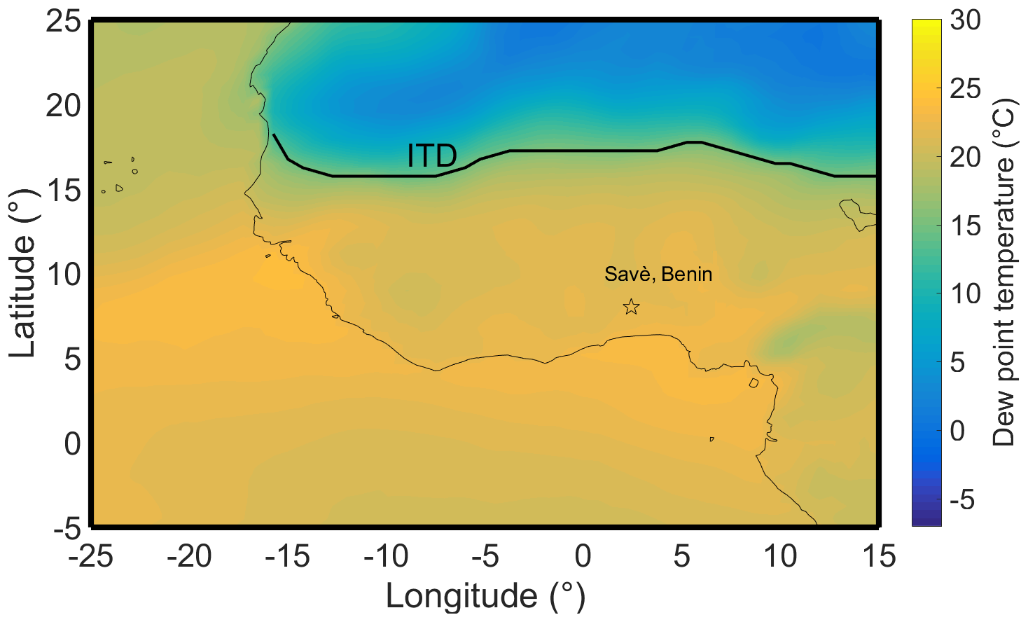
Figure 1Mean dew point temperature obtained from the ECMWF reanalysis at 2 m over southern West Africa during June 2016 and (solid black line) mean intertropical discontinuity (ITD) position during that month. The ITD position is deduced from the dew point temperature isoline of 15 ∘C. The star indicates the location of the Savè supersite.
Knippertz et al. (2017) also defined four synoptic phases of the monsoon using synoptic atmospheric circulations based on the precipitation difference between the coast (south) and the Sudanian–Sahelian zones (north):
- i.
Phase 1 (1–21 June) was a pre-onset phase characterized by the modulation of the winds and rainfall in the Guinea coastal area, due to three westward-propagating coherent cyclonic vortices between 4 and 13∘ N. The onset itself was associated with a breakdown of the African easterly jet, Saharan Heat Low, and rainfall due to an extratropical trough and cold surge over northern Africa.
- ii.
Phase 2 (22 June–20 July) was a post-onset phase characterized by a significant increase in low-level cloudiness and unusually dry conditions above. For example, around 12–14 July 2016, Knippertz et al. (2017) highlighted a rare situation of a cyclonic–anticyclonic vortex couplet that crossed southern West Africa (SWA). Unusually dry air was observed in SWA at that time, transported with the anticyclonic vortex which had its center in the Southern Hemisphere.
- iii.
Phase 3 (21–26 July) involved a westerly wind regime associated with wet conditions. During this phase, another vortex couplet, located a little further north than the previous one, enhanced westerly moisture transported into SWA.
- iv.
Phase 4 (27–31 July) was a phase of monsoon recovery characterized by undisturbed monsoon conditions.
A second very important dynamical feature is the NLLJ, which typically forms over land at the end of the day when turbulence in the atmospheric boundary layer has ceased. Blackadar (1957) associated the nocturnal jet with the ceasing of turbulence and predominance of the Coriolis force, which accelerates the wind towards low pressure. However, due to the low latitude and the low Coriolis force in the DACCIWA region, frictionless inertial oscillations above the nocturnal inversion layer might not be applicable. Therefore, the formation of the NLLJ may not be fully explained by this classical theory. Also observed during the AMMA experiment in the Sahelian region (Parker et al., 2005; Lothon et al., 2008; Abdou et al., 2010), the NLLJ settles almost every night in West Africa. Parker et al. (2005) suggested that when turbulence rapidly diminishes, the NLLJ is then able to respond to the pressure-gradient force.
Studies by Schrage and Fink (2012) and Schuster et al. (2013) have suggested that the NLLJ may play an important role in LLSC formation because of the cold air advection and turbulent mixing that it generates. Climate models tend to underestimate the strength of the NLLJ (Knippertz et al., 2011; Nam et al., 2012; Hannak et al., 2017) and consequently the advection and turbulent mixing that are associated with its occurrence. The NLLJ contributes differentially to horizontal advection as a function of latitude: transport of moisture occurs toward the north at high latitudes ( N) (Parker et al., 2005; Lothon et al., 2008). From the point of view of the DACCIWA region, transport by the NLLJ may be different. Due to the moisture gradient in SWA, which is characterized by less moisture over the Gulf of Guinea than inland, the NLLJ may actually transport drier air northwards, as revealed by Adler et al. (2019) and Babić et al. (2019a).
Another aspect of the DACCIWA region is the sea-breeze circulation that may be superimposed on monsoon flow around coastal regions. This circulation could have an impact on the transport of maritime air inland. Adler et al. (2017) and Deetz et al. (2018) used COSMO (Consortium for Small-scale MOdeling) simulations to show that the sea-breeze front, south of which the air is relatively cold compared with the northern more convective boundary layer, reaches several tens of kilometers inland during daytime convective conditions. After 15:00 UTC, with the weakening of convection and the associated turbulence, the wind increases and the front propagates further inland. Such a phenomenon was first studied along the Mauritanian coast and termed “Atlantic inflow” by Grams et al. (2010). Because this late afternoon propagation of the sea-breeze front occurs in a quite different context than that described by Grams et al. (2010), it is called Gulf of Guinea maritime inflow (here after MI) in the DACCIWA experiment (Adler et al., 2019) and is one of the processes involved in the LLSC formation during the DACCIWA field campaign (Adler et al., 2019; Babić et al., 2019a). Depending on the location of the sea-breeze front inland when it starts its late afternoon propagation, between 50 and 150 km must be traveled to reach Savè (Adler et al., 2019). Assuming a mean wind of 6 m s−1, this would mean that the MI should reach Savè between 19:00 and 21:00 UTC. Adler et al. (2019) and Babić et al. (2019a) studied the processes involved in the formation and evolution of LLSCs. They both highlighted the important role played by the MI and NLLJ within the monsoon flow diurnal cycle.
The present study aims to describe the day-to-day variability and mean characteristics of the monsoon flow, the NLLJ, the MI, and the LLSC at Savè, Benin (Fig. 1), during the 20 June–30 July 2016 period, based on the DACCIWA dataset. The focus on the Savè supersite for this study is motivated by the fact that only this site was instrumented in such way that continuous profiling of the wind up to several kilometers and continuous determination of the cloud summit were accessible. This was not the case at Kumasi or Ile-Ife. This investigation is a necessary step forward in ensuring a better understanding of the LLSC life cycle: this work should facilitate future case studies and the model evaluations. The subset of the instrumentation deployed at the Savè supersite and used in this study is described in Sect. 2. Section 3 provides the method and the criteria used to detect the monsoon flow. It overviews the day-to-day and mean characteristics of the monsoon flow. Section 4 presents the results for the NLLJ and MI, and Sect. 5 for the LLSC. Section 6 suggests a link between these three phenomena by presenting the mean diurnal cycle. A discussion and conclusions appear in Sect. 7.
During the DACCIWA field campaign, several remote sensing and in situ instruments were jointly deployed at Savè by the Karlsruhe Institute of Technology (KIT) and the Toulouse Paul Sabatier University (UPS). These instruments are all described in detail in Bessardon et al. (2019). The collected dataset has been presented in four published datasets: Handwerker et al. (2016), Kohler et al. (2016), Wieser et al. (2016) (for the KIT instrumentation), and Derrien et al. (2016) (for the UPS instrumentation). Furthermore, Kalthoff et al. (2018) give a comprehensive overview of the observations made at the three ground-based supersites of the DACCIWA projet, including Savè.
Below, we describe the instruments used in our statistical analysis, according to the object of study.
2.1 Wind profiling of the lower troposphere
An ultra-high-frequency (UHF) wind profiler operated by UPS was devoted to the study of the vertical structure of the atmospheric dynamics in the lower and middle troposphere. This 1274 MHz Doppler radar works with five beams. The three components of the wind are retrieved from these beams. This instrument was previously used for various studies of the planetary boundary layer: turbulence retrieval (Jacoby-Koaly al., 2002), African easterly jet analysis (Kalapureddy et al., 2010), the WAM diurnal cycle (Lothon et al., 2008), the NLLJ (Madougou et al., 2012), and offshore winds in high precipitation events (Said et al., 2016).
The radar ran continuously from 19 June to 30 July 2016 at Savè during the DACCIWA field experiment and provided vertical profiles of the wind every 2 min. We block averaged the data at 15 min time intervals for our wind analysis for consistency with other instruments. For our study, we considered the acquisition mode that corresponded to the highest radial resolution of 75 m, which enabled good documentation of the low troposphere from 150 m up to 3 km in height. The UHF profiler data are used here to characterize the monsoon flow, the NLLJ, and the MI.
2.2 Lower troposphere temperature profiling
A scanning microwave radiometer (humidity and temperature profiler HATPRO-G4 manufactured by RPG – Radiometer Physics GmbH) from the KIT was used to analyze the temperature profiles. The radiometer measured brightness temperature from which integrated water vapor, liquid water path, temperature profiles, and humidity profiles could be retrieved using the retrieval algorithm provided by the University of Cologne (Löhnert and Crewell, 2003; Löhnert et al., 2009). Every 15 min, temperature profiles with enhanced accuracy were obtained using low-elevation scans (Crewell and Löhnert, 2007), which are used here to detect the MI with the 302 K isotherm (Deetz et al., 2018) and the fuzzy logic algorithm described below. A systematic comparison of the radiosounding temperature profiles with the HATPRO temperature profiles (not shown) revealed a systematic cold bias of 0.2 K below 550 m, 0.5 K in the 550–1000 m layer, and 2 K in the 1000–2000 m layer. This finding is consistent with the accuracies noted by Crewell and Löhnert (2007) (<1 K below 1000 m). Only microwave radiometer measurements below 550 m are used in this study. The available dataset of this instrument covers the 30 June to 30 July time period.
2.3 Observation of surface layer conditions
A 7.77 m scaffold was mounted at Savè by UPS to study energy balance and biogenic fluxes. High-frequency measurements of air temperature, specific humidity, and three components of the wind were obtained (at 0.1 s time interval). The energy flux (latent heat, sensible heat, momentum flux) were calculated for the samples at a time resolution of 30 min. Additionally, upward and downward components of shortwave and longwave radiation, air pressure, soil temperature, and soil moisture were measured every minute.
This station operated continuously from 13 June to 30 July 2016. In this study, we use the sensible heat flux estimates to characterize the surface layer stability.
2.4 Cloud monitoring
Three co-located devices deployed during the DACCIWA field experiment are used to monitor low clouds: a ceilometer, cloud radar, and an infrared (IR) camera.
A CHM15k ceilometer, which is a 1064 nm wavelength lidar with a 5–7 kHz pulse rate, was installed by the KIT for the continuous monitoring of cloud base height (CBH). The ceilometer was operated from 3 June to 30 July 2016 at a time resolution of 1 min and a vertical resolution of 15 m. Manufacturer software automatically provided three estimates of CBH, which allowed us to detect multiple cloud layers. Here, we only use the lowest CBH, which corresponds to the low clouds under focus. We define “low-level clouds” as clouds with a base height below 1500 m a.g.l. Adler et al. (2019) used a lower altitude threshold, 600 m a.g.l., which is well adapted to the nocturnal stratus clouds. However, a 1500 m height limit allows us to extend our detection of LLSCs during daytime when the stratus cloud base height rises due to the growing convective boundary layer.
More information on cloud characteristics was provided by the KIT 35.5 GHz cloud radar (i.e., cloud top height (CTH) and cloud microphysics (rain, drizzle)). The cloud radar operated continuously from 14 June to 30 July 2016. It was run with vertical pointing every 5 min and horizontal scans every 30 min. Here, we use the observations of the vertical profiles for the CTH evaluation. After the despiking process, we averaged the reflectivity profiles of hydrometeors over 5 min and applied a threshold of −35 dBz to capture the CTH (Adler et al., 2019). Values below this threshold are considered to be related to clear air above the cloud. Additional details about the CTH retrieval technique can be found in Babić et al. (2019a). This algorithm enables a good estimation of the CTH, particularly when the clouds are uniform, which is true in the case of stratus clouds. However, CTHs are difficult to capture for scattered clouds or rain (e.g., cumulus clouds during the daytime). This fact explains some missing CTH estimates during the daytime in our later analysis. Finally, UPS installed a MOBOTIX S15 cloud camera that monitored the cloud cover all day and obtained visible and IR pictures every 2 min. The visible image was a full sky image: the aperture angles for the IR channel were (which corresponds to 158 m × 114 m in area at a height of 200 m). In this study, we used 5 MP IR images, coded in red, green, and blue (RGB) components over 256 colors. Here, [R,G,B] denotes the relative contributions of red, green, and blue of a given pixel, all defined between 0 and 1 (with accuracy of 1/256). The color of a pixel depends on the emissivity of the corresponding sky area and consequently its brightness temperature (uncalibrated). Typically, a low cloud base is seen as red and a clear sky is seen as blue. Therefore, a homogeneous low cloud deck will create a homogeneous red color image; a fragmented stratocumulus will render an image with colors ranging from red to blue. This instrument is used here to study the horizontal homogeneity of the cloud deck and to define the onset and breakup times of the stratus deck, with a newly designed method. As far as we know, it is the first time that such methodology is used for the study of stratus cloud deck formation and breaking.
3.1 Monsoon flow detection
The monsoon flow can be detected according to the wind direction (Kalapureddy et al., 2010). In this study, it is defined as the lower layer with a 135∘ (SE)–270∘ (W) horizontal wind sector. The choice to use a quite large wind direction sector, including some westerly winds, is motivated by weak monsoon flow (below 1 m s−1) observed during the daytime for which the direction is ill defined and can be influenced by local effects. This criterion on wind direction allows to exclude atmospheric conditions associated with vortex circulations, deep convection and Harmattan flow. The top of the monsoon flow is the level above which the horizontal wind direction is out of the 135–270∘ sector for more than 225 m (i.e., third UHF wind profiler gate). Very often, a large wind-sheared layer between the monsoon flow and the easterlies (African easterly jet) above is observed, which makes it difficult to determine the monsoon flow depth. The strength of the monsoon flow is defined as the mean wind speed within this depth.
3.2 Monsoon flow characteristics
Applying the previous criteria to the UHF wind profiler dataset, the temporal evolutions of the monsoon flow depth and strength from 15:00 UTC on day D-1 to 15:00 UTC on day D are calculated for day D from 20 June to 30 July 2016. The results are presented in Fig. 2. Except for 13, 16 and 17 July, dates for which the UHF wind profiler data are missing, the short periods shown in white in Fig. 2, are for a wind direction not falling within the 135–270∘ sector. As discussed in the previous section, the strong variability of the monsoon flow depth observed on some days, like 27–28 June, is associated with a large wind-sheared layer and a low wind. However, the intra-seasonal variability of the monsoon depth (from a few hundred meters to 4 km) and strength (from almost zero wind to 10 m s−1) can often be linked to synoptic conditions (Couvreux et al., 2010). Several days in a row, such as 20–23 June and 10–12 July, exhibited consistent monsoon flow characteristics over time with a particularly large monsoon flow depth and strong wind speed. The period 10–12 July is included in the vortex phase (9–16 July). During this period, an unusual cyclonic circulation developed and slowly propagated from eastern Mali to Cabo Verde along with an anticyclonic vortex in the west–northwesterly direction along the Guinean coast (Knippertz et al., 2017). The wet westerly regime (21–27 July) was characterized by a particularly low monsoon flow strength associated with important oscillations of the monsoon depth due to rain events that shifted back to the coast (Knippertz et al., 2017).
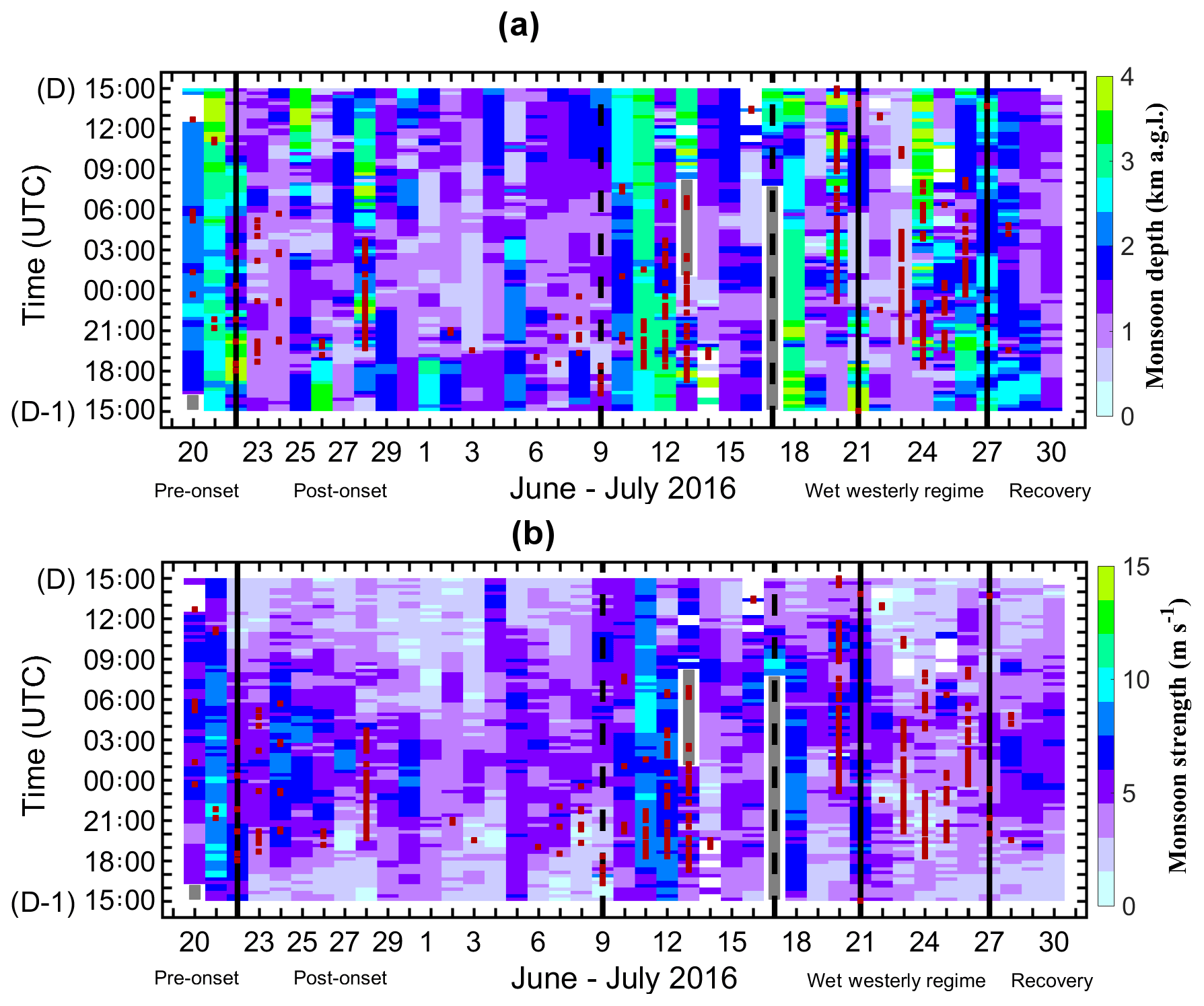
Figure 2Diurnal evolution of the monsoon flow (a) thickness and (b) strength at Savè from 15:00 UTC on day D-1 to 15:00 UTC on day D during the course of the 20 June through 30 July 2016 time period. Solid black vertical lines delimit the different phases of the monsoon described by Knippertz et al. (2017). Dashed vertical lines indicate the vortex phase included in the post-onset phase. White windows indicate periods for which the monsoon flow was not defined (i.e., a wind direction beyond the 135–270∘ sector). Grey windows indicate missing data. Red squares indicate rainy conditions.
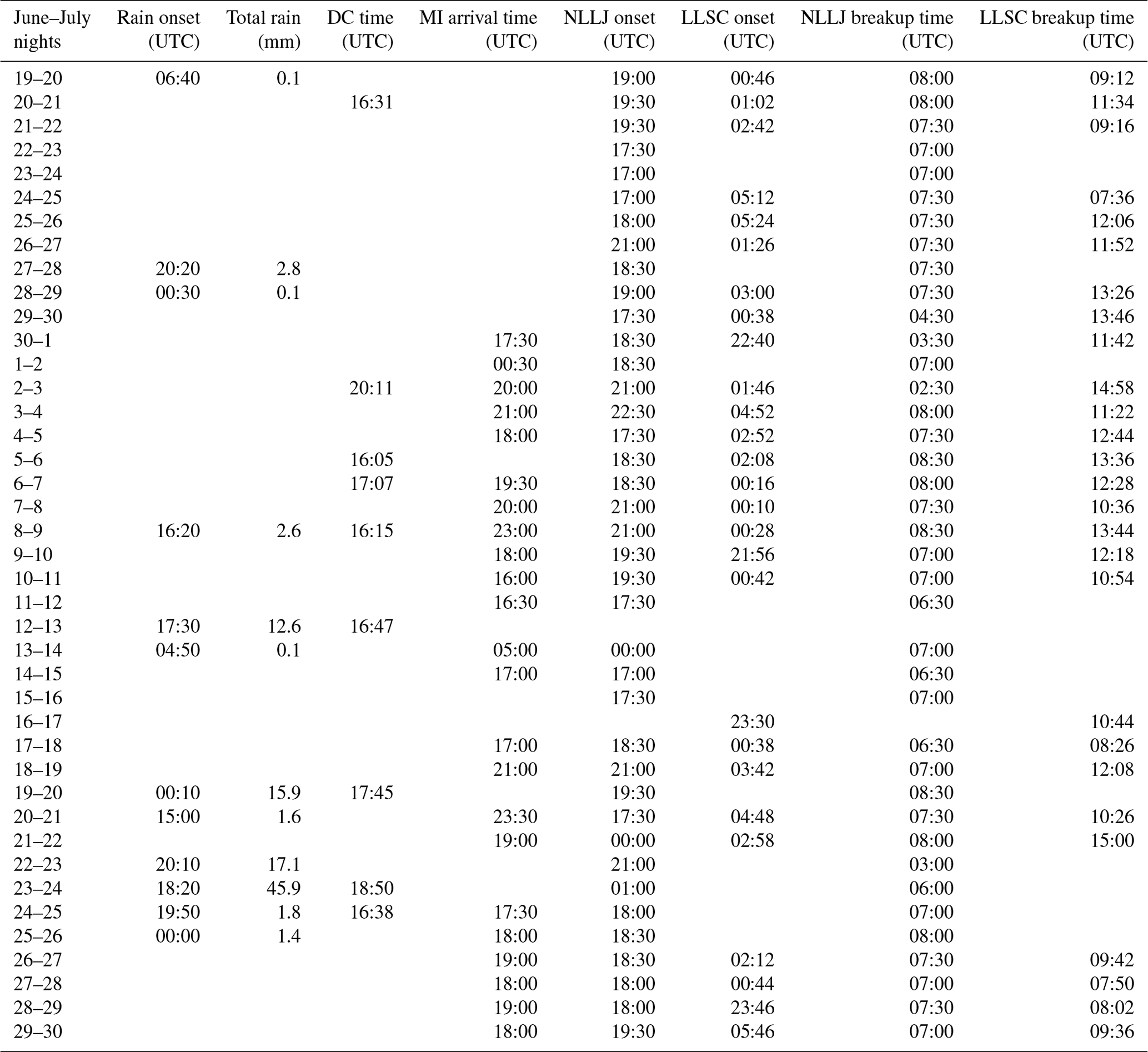
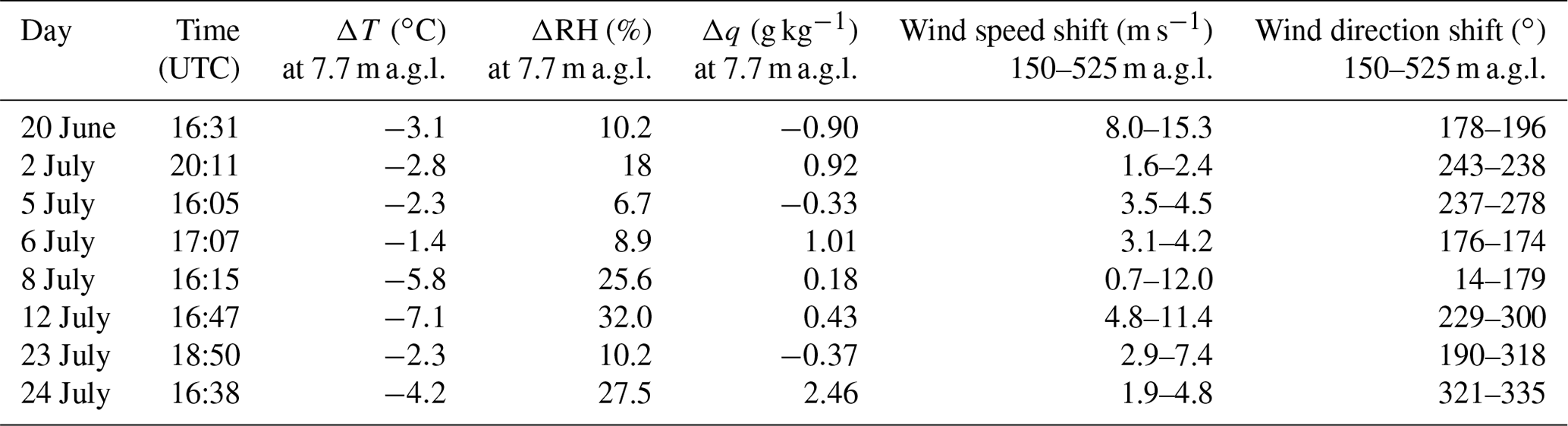
Many convective activities occurred at the Savè site during the campaign, which is typical in SWA (Laing and Fritsch, 1993). These phenomena were either detected by rain measurements (Fig. 2) or density current effects at the surface. Table 1 lists the days for which rain and/or density currents are detected after 15:00 UTC; such events are likely to have disturbed or interacted with the formation of LLSCs. The impact of density currents at the surface, in terms of temperature, relative humidity, specific humidity, wind speed, and direction depends on the intensity of the convective cell and its location. A sudden decrease in temperature and an increase in wind speed are typically observed (Table 2). A shift in wind direction is not a reliable criterion because it depends on the convective cell location with regard to the Savè supersite. As listed in Table 2, density currents are largely associated with drier air, as already discussed by Schwendike et al. (2010). All of the outflow cases listed in Table 1 are associated with a convective cell identified with the rain radar in the supersite surroundings. All of the rainy and density current cases are excluded (16 out of 41 d) from the statistics from which we estimate the primary characteristics of the monsoon flow.
Table 1Characteristics (onset and breakup time) of the NLLJ and LLSCs and the arrival time of the MI at Savé during the 20 June–30 July 2016 period. All times are indicated in UTC. For times related to the LLSCs, blanks indicate that LLSCs were not detectable (because of rain or clear sky). For times related to MI or NLLJ, blanks indicate missing data or undetectable features. The FLFmean was used to estimate the MI onset. DC indicates density current.
A composite 24 h evolution of the monsoon flow depth, strength, and direction from 15:00 UTC on day D-1 to 15:00 UTC the day after during the 20 June to 30 July 2016 period enables a discussion of the diurnal evolution of the monsoon flow characteristics (Fig. 3). The median of the monsoon depth shows a weak diurnal evolution from a minimum value of 1200 m a.g.l. during the night to 2000 m a.g.l. during convective conditions (Fig. 3a), with a day-to-day variability. This finding is consistent with what was observed during the AMMA experiment during the full monsoon season (Kalapureddy et al., 2010). Unlike the monsoon flow depth, the strength and direction of the monsoon flow indicate a clear diurnal cycle (Fig. 3b and c). The median strength of the monsoon flow is roughly 3.5 m s−1 between noon and 17:00 UTC with a 210∘ direction. The median strength regularly increases between 17:00 and 01:00 UTC up to 5.5 m s−1 with a simultaneous slight shift in the median wind direction (amplitude and standard deviation around 32.62 and 9.46∘, respectively). These same changes are observed in wind surface measurements (Kalthoff et al., 2018).

Figure 3Temporal evolution of the distribution of the monsoon flow (a) depth, (b) strength and (c) direction at Savè for the period between 20 June and 30 July. The black lines in panels (a), (b) and (c) indicate the median monsoon depth, strength, and direction, respectively.
4.1 Detection of the maritime inflow and nocturnal low-level jet
A low-level jet is characterized by a maximum wind speed a few hundred meters above the surface of the Earth and a clear minimum wind speed above. This situation implies significant shear below and above the jet core. Because of the occurrence of the low-level jets in various environments and forcing, different criteria can be applied to define and detect them based on vertical wind profiles. One of the first proposed definitions of the NLLJ based on observations was given by Bonner (1968). This author defined three types of NLLJs based on three different threshold values for the maximum wind speed (12, 16, and 20 m s−1, respectively), and the existence of a minimum wind speed above the maximum and below 3 km a.g.l. Stull (1988) and Andreas et al. (2000) defined the NLLJ within the first 1500 m as having a maximum wind speed at least 2 m s−1 faster than the minimum wind above it. Baas et al. (2009) defined NLLJs over the Netherlands as having a maximum wind speed at least 2 m s−1 below 500 m a.g.l. and a wind speed 25 % faster than the local minimum wind speed above.
The detection of the NLLJ is based, in this study, on the use of dynamical and surface stability criteria: (i) the wind direction in the lowest atmosphere below 1500 m is between the southeast and west–northwest with (ii) a maximum wind speed of at least 5 m s−1 and at least 2 m s−1 larger than the minimum above and (iii) a surface sensible heat flux lower than 10 W m−2. This last criterion ensures stable to neutral conditions at the surface. The onset of the NLLJ is defined when these criteria are satisfied for at least 2 h and the height of the maximum wind speed is below 500 m. The breakup time is defined when one of the three criteria mentioned above has not been satisfied for at least 1 h. The use of the surface sensible heat flux as a diagnostic of the stability may be a limitation to this method because this measurement is very local and may not represent atmospheric stability on large spatial scales. The NLLJ arrival and breakup times are determined with a 30 min temporal resolution, which corresponds to the sample duration for the sensible heat flux estimation.
The DACCIWA project focused on a region to the south of the AMMA study area that is affected by coastal phenomena, such as sea breeze. Unfortunately, no measurements provided evidence for MI formation and propagation inland. But based on simulations conducted by Adler et al. (2017) and Deetz et al. (2018), Adler et al. (2019) hypothesized that the MI penetrated 50–130 km inland. When convection and mechanical turbulence vanish at the end of the afternoon, two phenomena occur simultaneously: the monsoon flow increases and the MI, characterized by a higher wind speed than the monsoon flow further north, can propagate further inland, possibly up to Savè. Deetz et al. (2018), using COSMO model simulations for the night of 2–3 July, characterized the MI arrival by the 302 K potential temperature at a height of 250 m. This criterion was applied to the temperature measured locally by the microwave radiometer at the Savè site in order to detect the arrival of the MI. Since the 302 K criterion relies on one simulated case and because no clear justification for this 302 K value exists, another criterion based on MI characteristics observed at the surface is proposed in this study. MI arrival at Savè should be detected at the surface by a combination of both an increase in horizontal wind and a decrease in temperature. Thus, a second method was used in this study based on the combination of both an increase in horizontal wind speed and a decrease in temperature. These changes should be the signature of the MI arrival time. This method, based on the fuzzy logic method, was used by Coceal et al. (2018) to detect the sea-breeze front around London, in the south of England. Our method for MI detection at Savè follows three steps: (1) the rate of changes of temperature (T) and horizontal wind speed (ws) (termed rT and rws, respectively) are calculated using 30 min averaged T and ws in the 200–550 and 150–525 m layers, respectively; (2) fuzzy logic functions for T and ws, termed FLFT and FLFws, respectively, are computed using Eq. (1); and (3) the mean fuzzy logic function, FLFmean, combining both the changes in T and ws, is the mean of FLFws and FLFT.
The fuzzy logic function FLFx for the variable x can be written as
where rx is the rate of change of the variable x, (respectively, ) is a constant value below (above) which FLFx is equal to y1 (y2). rT is multiplied by −1 to obtain positive changes for decreasing temperature. As in Coceal et al. (2018), y1 and y2 are set to 0 and 1, respectively, and is set to 0 (i.e., no increase in wind speed or no decrease in temperature). Instead of using the maximum value of rx divided by two for (Coceal et al., 2018), for each day, we use the value corresponding to the 99th percentile of rx divided by two to avoid outliers. Considering the values used in this study for , y1, and y2 in Eq. (1) can be simplified as follows:
In this study, the mean fuzzy logic function (FLFmean) is computed using equal weights for FLFws and FLFT, and the same threshold of 1 is used to detect combined changes in the dynamic and thermodynamic conditions. The fuzzy logic method only makes sense if the temperature and wind speed changes are combined. However, to better understand how temperature and wind speed changes distinctly impact FLFmean, FLFws and FLFT are also discussed. FLFws would be a full weight applied to wind speed (i.e., considering that MI is only characterized by a dynamical change), and FLFT would be a full weight applied to temperature in the fuzzy logic method (i.e., considering that MI arrival implies only a thermodynamical change). The MI arrival time can then be determined by noting the first time at which the fuzzy logic functions of wind speed and temperature are equal to 1. There are, in this method, important constants and thresholds to fix, and several sensitivity tests have been performed. The results for individual days can differ, but the average and the conclusions remain the same.
The use of the MI and NLLJ criteria is illustrated for three very different days in Fig. 4. Each panel presents the 24 h time–height section of wind as measured by the UHF wind profiler and the three fuzzy logic functions (FLFws, FLFT, and FLFmean). The NLLJ onset times and the two estimates of the MI arrival time (302 K potential temperature and the fuzzy logic method) at Savè are also indicated.

Figure 4Time–height sections of (color) wind speed and (arrows) direction from the UHF wind profiler on the nights of (a) 2–3 July, (b) 7–8 July, and (c) 9–10 July 2016. A leftward horizontal arrow indicates an easterly wind; an arrow from bottom to top indicates a southerly wind. The black open circles indicate the jet core height detected with a maximum wind speed of at least 5 m s−1, the magenta rectangles indicate the height of the minimum wind speed above the jet core, and red open circles indicate the monsoon flow depth. The black, blue, and red lines in the lower box indicate the three fuzzy logic functions of the wind speed, temperature, and their mean, respectively. The red and black dashed vertical lines indicate the MI arrival time estimated using two different criteria: (1) the FLFmean>1 criterion and (2) the 302 K isentrope criterion, respectively. The black vertical line indicates the NLLJ onset.
A brief and weak NLLJ settled in the night of 2–3 July between 21:00 and 03:00 UTC in a very weak monsoon flow (Fig. 4a) and with a strong easterly wind above 2 km. The first simultaneous wind increase and cooling are observed at 20:00 UTC (FLFws, FLFT both reach 1), which indicates a clear MI arrival time. FLFmean values are larger than 0.5 until midnight, which demonstrates that the cooling lasts for at least 4.5 h. For that day, the 302 K potential temperature criterion is in very good agreement with the fuzzy logic method with a detection of MI arrival time at 20:15 UTC. The maximum value of the wind vertical profile reaches the threshold of 5 m s−1 at 21:00 UTC, which is the onset time of the NLLJ. The second example (Fig. 4b) is for the night of 7–8 July, which is analyzed in detail by Babić et al. (2019a). The fuzzy logic functions are very similar to those of 2–3 July. The estimated arrival times of the MI are 20:00 UTC and 20:45 UTC using the fuzzy logic method and the 302 K criterion, respectively. Like the night of 2–3 July, the maximum value of the jet reaches the threshold of 5 m s−1 at 21:00 UTC. The particularity of that day is that the NLLJ vanishes near the surface after sunrise on 8 July. However, the jet shape of the wind persists above unstable conditions; the height of the wind speed maximum increases up to 1000 m at 12:00 UTC which leads a strong rotation of the wind between the southwesterly in the monsoon flow and easterly above. This example illustrates the necessity of the atmospheric stability criterion for NLLJ breakup time determination. The third and last example, the night of 9–10 July (Fig. 4c), illustrates a NLLJ that was hardly detected because it develops within a strong monsoon flow observed all day long and weaker easterly wind above compared to 2–3 and 7–8 July. Six other days presenting a similar strong monsoon flow are observed during the period between 20 June and 30 July. These days correspond to synoptic anticyclonic atmospheric conditions over the Gulf of Guinea that favor a strong penetration of the monsoon flow inland (Knippertz et al., 2017). In such conditions, the NLLJ onset is not easy to determine. Figure 4c shows that the maximum wind is detected above 500 m before 19:30 UTC, which prevents us from considering this strong monsoon flow as a NLLJ until that time (criterion (i) of the NLLJ detection). The MI reaches Savè at 18:00 UTC according to the fuzzy logic method, 2 h earlier than the two previous examples. This result appears in accordance with a strong monsoon flow inhibiting the turbulent mixing and pushing the MI front faster and farther inland. On the other days, the cooling lasts until midnight. The detection of MI arrival time according to the 302 K criterion yields a later MI arrival time (19:30 UTC).
Based on these three examples, one can note the large variability that can be observed from one day to the other, which makes it challenging to define solid common criteria for MI and NLLJ detection.
4.2 MI and NLLJ characteristics
Characteristics of the MI and NLLJ are deduced from a set of days excluding rainy days and density current cases. For the NLLJ, we use the same days that we used for monsoon flow characteristics. For the MI, the 30 June through 30 July period is used (imposed by radiometer data availability), and 12 d are excluded (listed in Table 1).
Table 2Variations in surface (7.77 m height) temperature (ΔT), relative humidity (ΔRH), specific humidity (Δq), wind speed, and wind direction outflows that can disturb the MI arrival time and NLLJ onset and participate in the cooling of the atmosphere detected after 15:00 UTC. For the wind changes, the wind speed and wind direction averaged within the layer (150–525 m) before and after the event are considered.
The temporal occurrence of fuzzy logic functions equal to 1 for the 30 June–30 July period is shown in Fig. 5. One can note interesting results:
-
A large increase in wind speed (FLFws=1) may be observed at any time during the day; however, the largest occurrence (≥5) is between 17:00 and 20:00 UTC. This variability is due to the day-to-day variability of the monsoon strength and the arrival time of the NLLJ during this period.
-
As expected, cooling may occur between 18:00 and 00:30 UTC the following day. Contrary to the wind speed, whose fuzzy logic function reaches 1 but rarely remains at that value for several hours during the night, the temperature fuzzy logic function reaches this value many times during the night. This trend implies continuous cooling (Fig. 4). This result is in accordance with the continuous decrease in temperature within the MI from north to the south discussed by Adler et al. (2019). A large abrupt change in temperature at the front passage with constant temperature behind would have implied a very different temporal occurrence of FLFT=1. In addition, the continuous cooling can also be explained by the turbulent mixing under the NLLJ core, which mixes the upper layer with lower layers cooled by radiative and sensible flux divergence (Adler et al., 2019; Babić et al., 2019a).
-
The FLFmean with values equal to 1 combines the wind increase and the cooling, both of which occur simultaneously during the entire night; the largest number of cases is observed between 18:00 and 21:00 UTC.
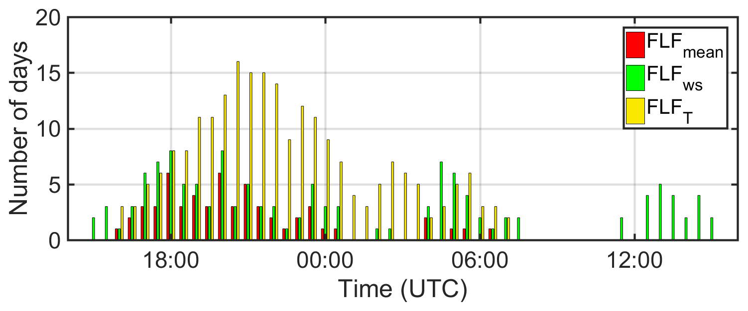
Figure 5Temporal occurrence of fuzzy logic functions equal to 1 for temperature (FLFT), wind speed (FLFws), and mean fuzzy logic function (FLFmean) for the period between 1 and 30 July.
The MI arrival times are shown in Fig. 6a. Four estimates of the MI arrival times are displayed, one using the 302 K potential temperature criterion and three corresponding to the first time when the three fuzzy logic functions, FLFws, FLFT and FLFmean, attain a value of 1. Most of the observations of the MI arrival time at Savè considering only the wind speed increase fell between 16:00 and 18:00 UTC, while they fell between 16:00 and 21:00 UTC when we considered only the cooling. The arrival time of the MI deduced from FLFmean, which couples with an equal weight cooling and wind speed increase, is observed between 16:00 and 00:00 UTC, with a median arrival time at 19:00 UTC. As noted above, the different tests performed to select the constants and thresholds for the fuzzy logic method yield different MI detection times for each day but quite similar distributions for the period of study. These results suggest that the MI arrival time is difficult to detect with local measurements. However, the MI arrival time as detected by the fuzzy logic function FLFmean is clearly linked to the mean monsoon flow in the afternoon (Fig. 7): the stronger the monsoon flow strength in the afternoon between 12:00 and 15:00 UTC, the earlier the MI arrival time. The absolute value of the correlation coefficient between both is 0.61. The two exceptionally early arrivals at 16:00 and 16:30 UTC shown in Fig. 7 and put in Table 1 are associated with unusually strong monsoon flow all day long (e.g., the nights of 10–11 and 11–12 July).

Figure 6(a) Distribution of MI arrival times determined using the 302 K potential temperature criterion and the fuzzy logic function method (FLFT, FLFws, and FLFmean) for the period between 1 and 30 July 2016. (b) Distribution of NLLJ onset and breakup times at Savè during the period from 20 June to 30 July 2016. The MI arrival times detected with FLFmean, already presented in panel (a), are also indicated.
The NLLJ onset and breakup cannot be detected prior to 17:00 UTC and after 08:00 UTC, respectively, because of the stability criterion. The most frequent onset and breakup times of the NLLJ are 17:30 and 07:00 UTC, respectively (Fig. 6b). The MI arrival time detected with FLFmean=1, is also indicated in Fig. 6b. One can note that, with the exception of the two exceptionally early MI arrival times, the NLLJ onset and MI arrival time distributions are quite similar to one another. Table 1 summarizes, for each day of the 20 June through 30 July period, the MI arrival time using FLFmean, NLLJ onset and breakup times, in addition to the rainy and density current cases noted before.
Figure 8 shows a 15 min distribution of the jet core height, strength, and direction for the 20 June through 30 July period. The median jet core lowest height (350 m) is observed when the NLLJ settles. The jet core rises after 22:00 UTC to reach about 500 m at NLLJ breakup. The median strength of the jet varies between 7 and 11 m s−1 (Fig. 8b), and the median direction shifts slightly from 200∘ at NLLJ onset to 230∘ at 03:00 UTC (Fig. 8c). The NLLJ core in Niger and Benin observed during the AMMA campaign (Lothon et al., 2008) was roughly at the same height, but the wind speed of the jet core is in contrast more pronounced in Niger, from 10 to 20 m s−1.
5.1 LLSC detection
West African LLSCs have not been extensively studied in the past, generally due to a lack of observations. However, the systematic visual observations by local meteorologists at every meteorological station made over a time period of years constitute a unique dataset (Schrage and Fink, 2012). Besides this historical approach, several instruments have been used in the context of international projects to estimate LLSC characteristics from a vertical point of view: radiosoundings, cloud radar (Bouniol et al., 2012), and ceilometer (Schrage and Fink, 2012). Satellite data have also been used to analyze the horizontal variability LLSCs. Van Der Linden et al. (2015) and Bouniol et al. (2012), for example, made a climatology of the occurrence of the LLSCs in this region.
Here, we use a ceilometer to estimate the CBH (considering only CBHs below 1500 m a.g.l.), cloud radar to estimate the CTH and the IR sky camera to define the start and end of the LLSCs (Sect. 2.4). With the IR sky camera, we have the advantage of retrieving information about the occurrence of LLSCs, as well as their horizontal structure on a local scale.
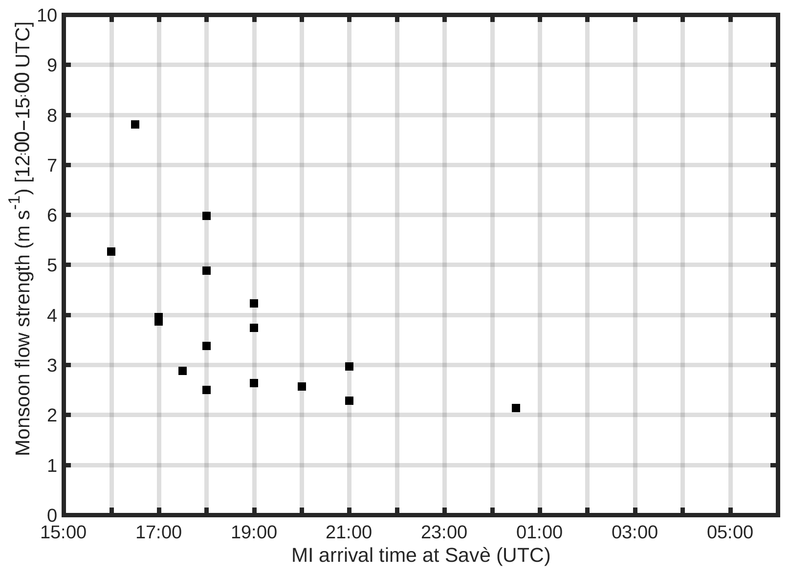
Figure 7Scatter plot of the average monsoon strength between 12:00 and 15:00 UTC and the MI arrival time using FLFmean=1, for the time period between 1 and 30 July 2016.
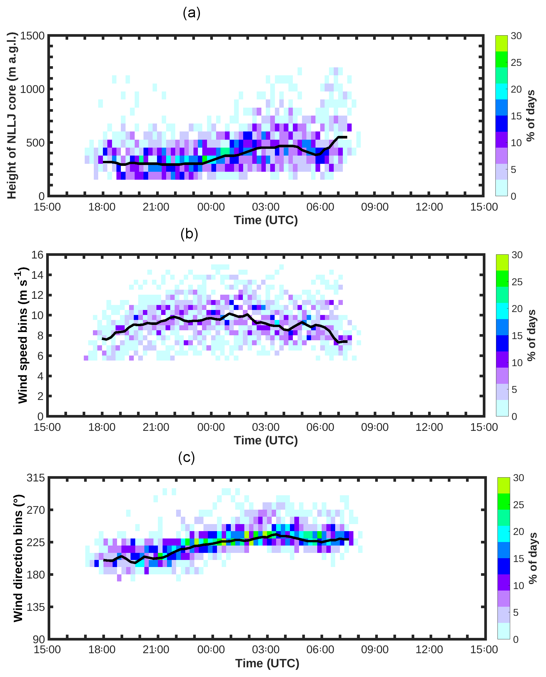
Figure 8Distribution of the NLLJ (a) core height, (b) strength, and (c) direction at the Savè supersite. The color bar indicates the percentage of days (computed using the number of nights with NLLJ onset during the 20 June through 30 July period). The black lines in panels (a), (b), and (c) indicate the median jet core height, its strength, and its direction, respectively.
To estimate the occurrence of stratus clouds at Savè, we consider the average color defined by the color vector obtained when averaging all [R,G,B] pixels of the IR camera image, as well as the standard deviation σRGB. σRGB quantifies the color variability within each image, which represents the spatial variability of the lowest CBH within the aperture:
where σR, σG, and σB are the standard deviations of the , , and components, respectively, within the image.
A large standard deviation implies a large variability of temperature (i.e., a mix of clear sky and clouds) or spatial variability of the CBHs; a small standard deviation corresponds to either a homogeneous stratus deck or a fully clear sky.
Here, we set the occurrence of the low stratus clouds when (i) , , and , (ii) , for more than 2 h without any “break” longer than 30 min. Furthermore, the first time when these criteria are satisfied should occur before 06:00 UTC the following morning in order to detect only nocturnal LLSCs. The first criterion (i) corresponds to the search of a low base, with an average color close to red. The second criterion (ii) corresponds to the search for a relatively homogeneous cloud deck. The added persistence condition helps with defining a consistent nocturnal stratus cloud life cycle and avoids spurious variability. These criteria allow one to estimate, for each night, the onset and breakup times of LLSCs and therefore deduce their lifetimes. Note that during rain events, droplets are retained on the dome of the infrared camera and impact the color of the image as if there was a cloud. Therefore, LLSCs cannot be detected during rain events which are thus excluded. As far as we know, it is the first time that such methodology is used for the study of the stratus cloud deck formation and breaking.
Figure 9 shows two typical examples to illustrate this method using information provided by the ceilometer and the cloud radar. The evolution of the average color and the standard deviation during two nights (the nights of 7–8 July and 6–7 July are shown in Fig. 9a and b, respectively) are shown with the CBH estimated from the ceilometer and the CTH estimated from the cloud radar. Onset and breakup times deduced when applying the detection method are also indicated.
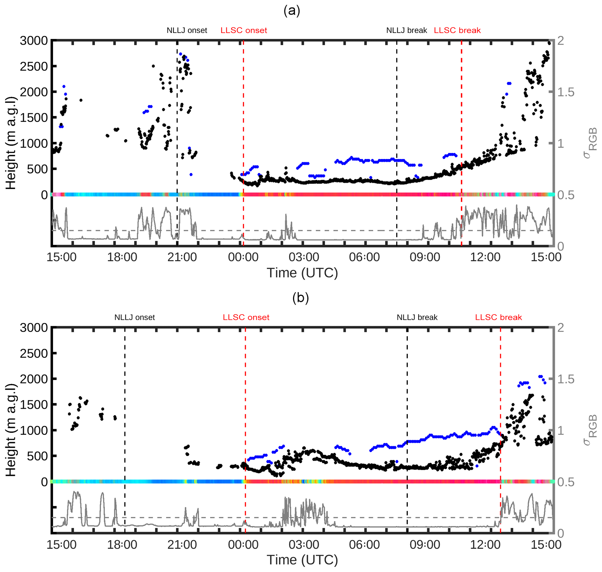
Figure 9Time series of the LLSC macrophysical characteristics observed on the nights of (a) 7–8 July 2016 and (b) 6–7 July at Savè. The colored band indicates the time series of the average image obtained every 2 min with the IR cloud camera. This time series is plotted arbitrarily at the 0 m abscissa for the sake of clarity. The grey line indicates σRGB (with its scale on the right axis) and the dashed grey line indicates for the threshold (0.15) above which the LLSC deck is not considered to be homogeneous. Black dots indicate the CBHs of the LLSCs estimated from the ceilometer. Blue dots indicate the CTHs of the LLSCs estimated from the cloud radar. The dashed black and red vertical lines indicate from left to right the NLLJ and LLSC onset and breakup times.
For both examples, one can see how the smallest steady standard deviation of the IR image color consistently corresponds more to a steady low cloud base as seen by the ceilometer (see, for example, the data from 8 July from 03:00 to 08:00 UTC or the data from 7 July from 06:00 to 09:00 UTC). A larger standard deviation corresponds to more variability of the cloud base (e.g., on 8 July around 11:00 UTC or 7 July around 03:00 UTC or after 12:30 UTC).
For the night of 7–8 July (Fig. 9a), the criteria for LLSC detection are satisfied from midnight until 10:30 UTC. This period defines the LLSC lifetime for this day (Table 1). Before midnight, the sky is clear for a large part of the time (blue color with the IR camera); some clouds passed between 10:00 and 15:00 m a.g.l. The cloud base heights are variable according to the ceilometer; the IR color and σRGB do not satisfy the LLSC detection criteria. After 10:30 UTC, the cloud base rises and the fractionation of the cloud base (less steady red–pink color; large σRGB for a long duration of time) increases with the development of the convective boundary layer. It defines the end of the stratus. We consider the preceding lifting of the stratus deck from 07:30 to 10:30 UTC as being part of the LLSC lifetime (i.e., they meet our criteria for LLSC detection), which is the start of the so-called “convective phase” according to Babić et al. (2019a), who focused on the night of 7–8 July 2016 in their case study, and Lohou et al. (2019), who suggested a conceptual model of LLSCs' life cycle.
For the night of 6–7 July, the criteria for stratus LLSC are satisfied from slightly after midnight until 12:30 UTC (Table 1). The variability of cloud base found between 02:00 and 04:00 UTC, and revealed by higher σRGB and smaller values, does not persist long enough to interrupt the LLSC definition.
Adler et al. (2019) used the ceilometer to estimate nocturnal LLSC characteristics (CBH, onset, and breakup times). These authors differentiated between LLSC stratus deck and preceding “stratus–fractus” phase using two lower-bound thresholds of 90 % and 50 %, respectively, for the cloud fraction computed within a 60 min time interval. An example of those two phases can be seen on the night of 6–7 July (Fig. 9b). One can see that low clouds occur between 21:00 UTC and midnight; they have a slightly higher base than later in the night, and there are long periods without clouds. This phase corresponds to the stratus–fractus phase defined by Adler et al. (2019), which precedes the “stratus phase”. Due to our criteria related to the persistence of LLSCs, this phase is excluded from our detection method. We instead detect the “stratus phase” that corresponds to full-deck LLSCs. Note that a very short stratus–fractus phase can also be seen in the previous example of the night of 7–8 July (Fig. 9a), from 23:30 to 00:10 UTC, which is also consistent with the work of Adler et al. (2019) and Babić et al. (2019a).
Clouds after 12:00 UTC for both cases correspond to convective shallow cumulus (within the “convective phase” noted by Babić et al., 2019a), as revealed by both a larger IR image standard deviation (σRGB) and the very large scatter in the ceilometer-based CBH between 1000 and 3000 m a.g.l. (Fig. 9). The formation of cumulus clouds below the LLSCs is one of the three LLSC breakup scenarios described in Lohou et al. (2019), but the shallow cumulus and fair weather cumulus are not detected by our criteria and indeed not under scope here.
5.2 LLSC lifetime statistics
Based on the detection criteria explained above, we noted a significant occurrence of LLSCs during the DACCIWA campaign at Savè: 65 % of the nights exhibit the development of a nocturnal stratus deck. This finding is consistent with the work of Kalthoff et al. (2018).
This prevalent occurrence is revealed in Fig. 10, which shows, from 15:00 UTC one day (D-1) to 18:00 UTC the following day, the MI arrival time and onset and breakup times of LLSC and NLLJ.
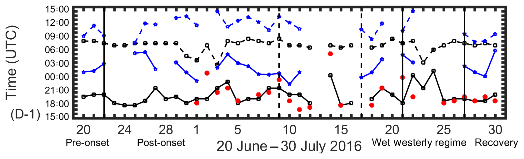
Figure 10The time series of the onset (solid lines) and breakup times (dashed lines) of NLLJ and LLSCs are shown in black and blue, respectively. The red colored circles indicate the arrival time of the MI at Savè using the mean fuzzy logical function. Solid black vertical lines delimit the different phases of the monsoon described by Knippertz et al. (2017). Dashed vertical lines indicate the vortex phase included in the post-onset phase.
Figure 10 shows some intra-seasonal variability. The pronounced occurrence of LLSCs from 26 June through 11 July corresponds to the post-onset phase of the WAM. It is interrupted from 12 to 17 July by the drier vortex period identified by Knippertz et al. (2017) and noted above. From 23 to 26 July, the westerly moist regime observed (not shown here but seen in the UHF wind profiler data of Kalthoff et al., 2018) is associated with more rain (nearly on a nightly basis). This situation prevents LLSCs from being detected using the sky camera.
The shortest lifetime of the LLSCs was observed on 30 July. On this day, the onset LLSC is observed very late. For some cases, the breakup time is observed after noon, as on 3 July. A large variability in LLSC characteristics is observed: some nights exhibit steady LLSCs, and other nights have lots of intermittent LLSCs (figure not shown) (e.g., 11, 21, 29 July). On the days that LLSCs form, they appear usually more than 3 h after the onset of the NLLJ and clear up after the NLLJ breakup time (Fig. 10).
Figure 11 gives more quantification of those time characteristics. It displays the distribution of the LLSC onset time and breakup time over the same set of 25 selected days as the monsoon flow statistics discussed above. Large variability in onset and breakup times of LLSCs is indeed observed. Overall, 26 % of LLSC onsets are observed before 00:00 UTC, and 78 % are observed before 03:00 UTC. All breakup times are observed after sunrise: 33 % of LLSC breakup times occurred before 10:00 UTC, and 74 % occurred before 12:00 UTC. We found that LLSCs always clear up after the NLLJ breakup time.
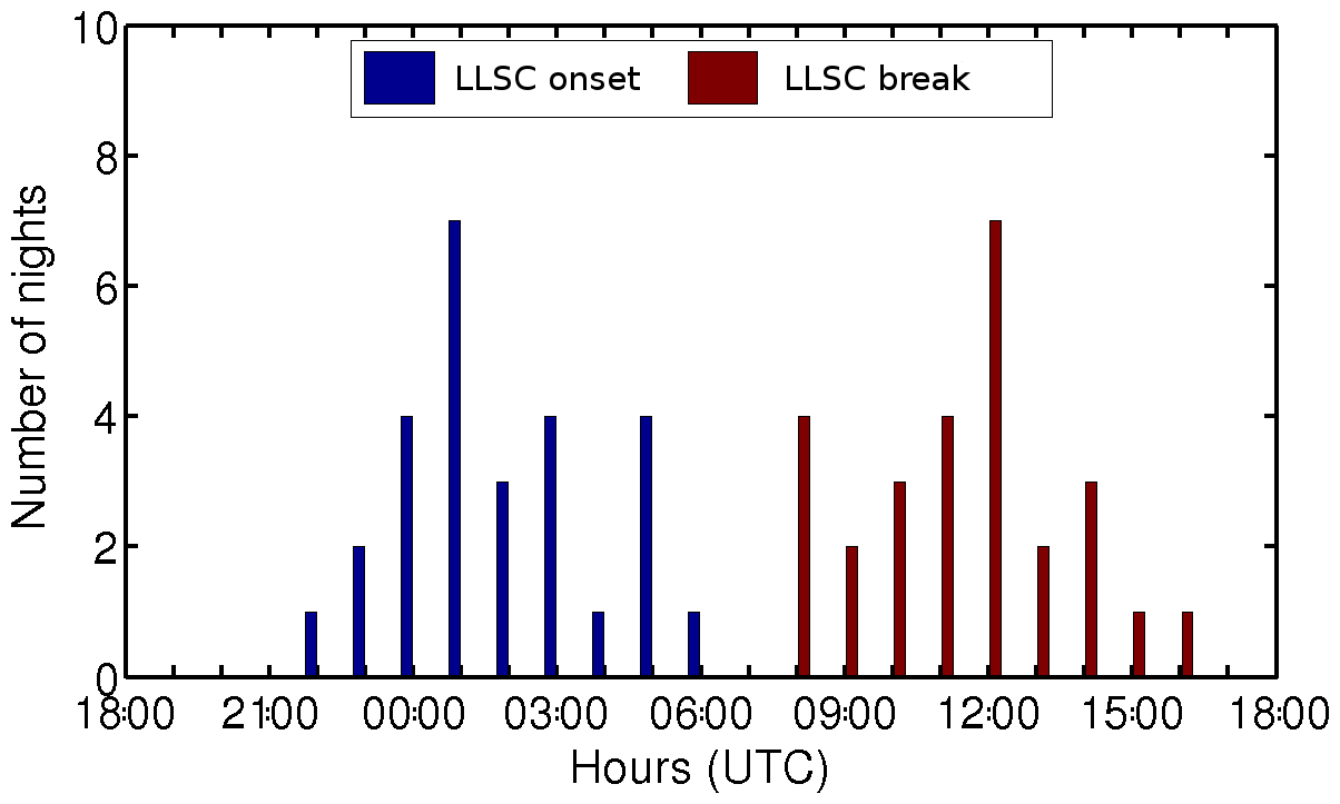
Figure 11Distribution of (blue) onset and (brown) breakup times of LLSCs at Savè from the period of 20 June through 30 July 2016.
Based on the detection of the NLLJ and LLSCs discussed before, we now discuss their composite diurnal cycle.
Figure 12 shows the composite diurnal cycle of the NLLJ core height, LLSC base height, and LLSC top height computed using the median of those diagnostics over all considered days as indicated previously. The shaded areas correspond to the standard deviation of the ensemble. Note that calculations of the median and standard deviation are possible only when more than five cases can be taken into account. Thus, for the NLLJ core height, between 10 and 25 d are taken into account between 18:00 (D-1) and 06:30 UTC. For the CBH, between 10 and 25 d are taken into account from 00:00 to 11:40 UTC. For the CTH, between 10 and 25 d are taken into account between 04:00 and 11:20 UTC.
Figure 12 provides a schematic evolution of the NLLJ and of the LLSCs that we observe during the DACCIWA field experiment at the Savè site for the 25 d considered in the statistics.
The median NLLJ core height remains lower than 350 m a.g.l. until the onset of the LLSC. Once the LLSC starts to form, the NLLJ core rises within the stratus clouds until it dissipates in the morning with increasing instability. LLSCs of 340±90 m thickness form on average at the NLLJ core height. This average thickness is very similar to that found by Adler et al. (2019) based on all days of the intensive observation period (340±80 m, over 11 IOP (intensive observation period) days). The CBH is usually stationary during the night from 00:00 to 06:00 UTC. It sharply increases after 08:00 UTC when the convective boundary layer develops.
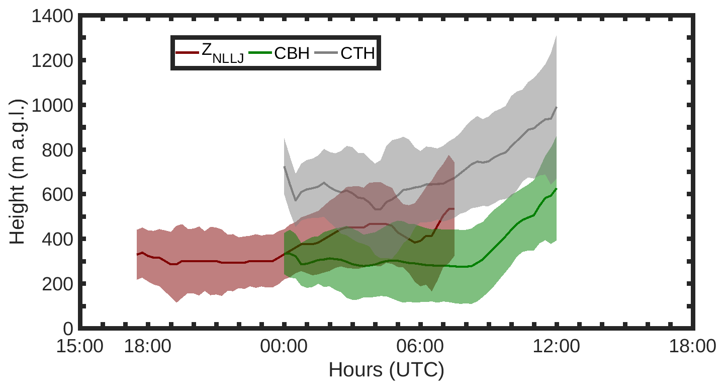
Figure 12Median diurnal cycle of the NLLJ core height (solid red line), cloud base height (solid green line) and cloud top height (solid grey line) from 20 June to 30 July 2016 at the Savè supersite. Shaded areas indicate variability (±σ).
An analysis of a 41 d DACCIWA dataset during the WAM in 2016 in Benin enabled a quantified documentation of low-level stratiform clouds and dynamical structures in the low troposphere. A key need for observations to compare with numerical weather and climate models motivated the field campaign in the DACCIWA project.
The months of June and July in West Africa are characterized by deep convection, and the conditions at Savè supersite are frequently disturbed by MCSs. Among the 41 d period, 16 d have been excluded from the quantified statistics. However, many other MCSs may have impacted the flow between the coast and Savè without being detected at Savè. These MCSs are an important part of the monsoon in West Africa and participate in the variability of the low-level cloud and dynamical structures discussed below. When they occurred in the surroundings of the Savè site, MCSs could be detected (rainfall or density current) and excluded from the analyzed days. However, MCSs occurring upstream of Savè were hard to detect and could have some more subtle impacts on the monsoon flow or the MI characteristics or propagation.
The intra-seasonal variability of the synoptic situation analyzed by Knippertz et al. (2017) impacts not only the monsoon flow depth and intensity but all low troposphere structures. For example, a break of the WAM activity in mid-July with an unusual cyclonic dry air mass circulation weakened the monsoon flow and the NLLJ and inhibited LLSC formation at Savè (Babić et al., 2019b). Besides the day-to-day variability of the monsoon flow due to large-scale atmospheric conditions, the median diurnal cycle of the monsoon flow exhibits a 1500 m depth southwesterly monsoon flow of 6 m s−1 at night, which slightly deepens (2000 m), slows down (4 m s−1), and becomes more southerly during the day.
The advection of cool air at Savè is due to two processes already noted by Adler et al. (2019) and Babić et al. (2019a): MI and the NLLJ. The two processes occur because of the late afternoon decrease of the turbulence due to convection. Considering the MI propagation time to reach Savè, both processes are hypothesized to be observed at Savè between 17:00 and 21:00 UTC. The MI is rather unknown and poorly observed, but its passage at a given location is expected to imply an increase in the wind speed and a decrease in the temperature. The fuzzy logic method applied in this study to detect the MI arrival time leans on these expectations and depends on the weight attributed to the changes in temperature and wind speed. The NLLJ has been extensively studied in different places around the world but the detection of its time settlement is for sure a question of criteria, particularly the threshold for the wind jet core (5 m s−1 in this study). Despite these inherent limitations of criteria-based methods, MI arrival and NLLJ settlement times are estimated at Savè in June and July 2016. The MI arrival time at the Savè site occurs between 16:00 and 21:00 UTC; the median occurrence time is at 19:00 UTC. The NLLJ is a systematic feature within the monsoon flow, with a jet core wind speed between 7 and 11 m s−1 within the (200–300∘) southwesterly sector at a height of about 350 m. It usually sets up before 21:00 UTC (median time occurrence is 18:30 UTC) and ceases before 07:00 UTC.
The large time range for MI arrival time at Savè is due to the large range of monsoon flow strength 1–5 m s−1 with few cases above 6 m s−1. It also depends on the capability of the turbulent mixing to balance monsoon flow, which slows the front progression in land. The MI arrival time is then concomitant with the NLLJ onset; the two processes, as we defined them in this study, are sometimes difficult to distinguish. The acceleration of the monsoon flow through the NLLJ over West Africa causes the ITD to penetrate about 100 km further north every night (Pospichal and Crewell, 2007; Lothon et al., 2008). It is plausible that the MI contributes to this process as well; the Gulf of Guinea/continent contrast and breeze front may come into play as well.
Using an infrared cloud camera, an original methodology is defined to detect the onset and breakup time of the low-level stratiform cloud over Savè. Based on this instrument, the results show that the low-level stratus is a persistent phenomenon that occurs 65 % of nights during our studied period. It forms more than 3 h (6 h on average) after the NLLJ onset at the jet core height and persists until noon on 80 % of days with nocturnal stratus formation. Our diagnostics on NLLJ and LLSC characteristics gave a good representation of the diurnal cycle of the lowest atmosphere conditions observed over the southern part of West Africa. We have shown that LLSCs form at around 00:00 UTC with their base at the same height as the NLLJ core. The LLSC base and top heights remain constant during the night (340 m thickness) and rise as the cloud deepens during early morning. LLSCs persist until early afternoon.
The results of our study reveal how closely related NLLJ, MI, and LLSC phenomena are. The processes involved in the LLSC formation and related to the MI and NLLJ are addressed in Adler et al. (2019) and Babić et al. (2019a), and a conceptual model of the LLSC life cycle proposed in Lohou et al. (2019). The present study brings an overall statistical analysis of the key dynamical features of the low troposphere during the WAM. It also intends to show the day-to-day variability and exhaustively gives quantified diagnostics for each day of the entire period. Therefore, it is an important basis for any future case study. Moreover, these results can be used for model evaluation. A special focus could be given to the NLLJ simulation since the NLLJ has been shown to play an important role in the air cooling and shear-driven turbulence prior to the saturation and LLSC formation.
The DACCIWA embargo period is over; the data of the Savè supersite are available on the baobab database (https://doi.org/10.6096/dacciwa.1618, Derrien et al., 2016; https://doi.org/10.6096/dacciwa.1686, Handwerker et al., 2016; https://doi.org/10.6096/dacciwa.1690, Kohler et al., 2016; https://doi.org/10.6096/dacciwa.1659, Wieser et al., 2016) for scientists interested in boundary-layer studies in southern West Africa (http://baobab.sedoo.fr/DACCIWA, OMP, 2019).
CD, FL, ML, NK, BA, YB, OG, and XPB participated in the DACCIWA campaign and data processing. CD prepared the manuscript with contributions from all co-authors.
The authors declare that they have no conflict of interest.
This article is part of the special issue “Results of the project “Dynamics-aerosol-chemistry-cloud interactions in West Africa” (DACCIWA) (ACP/AMT inter-journal SI)”. It is not associated with a conference.
The DACCIWA project has received funding from the European Union Seventh Framework Programme (FP7/2007-2013) under grant agreement no. 603502. The authors thank also Laboratoire d'Aérologie, Université de Toulouse, CNRS, UPS, France, and KIT (Karlsruhe Institute of Technology) and UPS (Université Toulouse) for helping to install the equipment, as well as the people from INRAB in Savè for allowing the equipment on their ground. We thank the Aeris data infrastructure for providing the DACCIWA Operation Center during the campaign and the access to the data used in this study.
The research leading to these results has received funding from the European Union Seventh Framework Programme (FP7/2007-2013) under grand agreement no. 603502.
This paper was edited by Susan van den Heever and reviewed by Michael Diamond, Christophe Lavaysse, and one anonymous referee.
Abdou, K., Parker, D. J., Brooks, B., Kalthoff, N., and Lebel, T.: The diurnal cycle of lower boundary-layer wind in the West African monsoon, Q. J. Roy. Meteor. Soc., 136, 66–76, https://doi.org/10.1002/qj.536, 2010. a
Adler, B., Kalthoff, N., and Gantner, L.: Nocturnal low-level clouds over southern West Africa analysed using high-resolution simulations, Atmos. Chem. Phys., 17, 899-910, https://doi.org/10.5194/acp-17-899-2017, 2017. a, b
Adler, B., Babić, K., Kalthoff, N., Lohou, F., Lothon, M., Dione, C., Pedruzo-Bagazgoitia, X., and Andersen, H.: Nocturnal low-level clouds in the atmospheric boundary layer over southern West Africa: an observation-based analysis of conditions and processes, Atmos. Chem. Phys., 19, 663–681, https://doi.org/10.5194/acp-19-663-2019, 2019. a, b, c, d, e, f, g, h, i, j, k, l, m, n, o, p
Andreas, E. L., Claffey, K. J., and Makshtas, A. P.: Low-level atmospheric jets and inversions over the Western Weddell Sea, Bound.-Lay. Meteorol., 97, 459–486, 2000. a
Baas, P., Bosveld, C., and Klein Baltink, H.,and Holtlag, A. A. M.: A climatology of Nocturnal Low-Level Jets at more frequent occurrence of the LLC during the monsoon Cabauw, J. Appl. Meteorol. Clim., 48, 1627–1642, 2009. a
Babić, K., Adler, B., Kalthoff, N., Andersen, H., Dione, C., Lohou, F., Lothon, M., and Pedruzo-Bagazgoitia, X.: The observed diurnal cycle of low-level stratus clouds over southern West Africa: a case study, Atmos. Chem. Phys., 19, 1281–1299, https://doi.org/10.5194/acp-19-1281-2019, 2019a. a, b, c, d, e, f, g, h, i, j, k
Babić, K., Kalthoff, N., Adler, B., Quinting, J. F., Lohou, F., Dione, C., and Lothon, M.: What controls the formation of nocturnal low-level stratus clouds over southern West Africa during the monsoon season?, Atmos. Chem. Phys. Discuss., https://doi.org/10.5194/acp-2019-537, in review, 2019b. a
Bessardon, G., Brooks, B., Abiye, O., Adler, B., Ajao, A., Ajileye, O. Amekudzi, L. K., Armah Aryee, J. N., Atiah, W. A., Ayoola, M., Bret, G., Bezombes, Y., Cayle-Aethelhard, F., Danuor, S., Delon, C., Derrien, S., Dione, C., Durand, P., Brilouet, P. E., Fosu-Amankwah, K., Gabella, O., Groves, J., Handwerker, J., Kalthoff, N., Kohler, M., Kunka, M., Jambert, C., Jegede, G., Leclercq, J., Lohou, F., Lothon, M., Medina, P., Pedruzo, X., Reinares, I., Sharpe, S., Smith, V., Sunmonu, L., Tan, T., and Wieser, A.: A new high-quality dataset of the diurnal cycle of the southern West African atmospheric boundary layer during the Monsoon season – an overview from the DACCIWA campaign, Sci. data., in review, 2019 a, b
Blackadar, A. K.: Boundary layer wind maxima and their significance for the growth of nocturnal inversions, B. Am. Meteorol. Soc., 38, 283–290, 1957. a
Bonner, W. D.: Climatology of the low level jet, Mon. Weather Rev., 96, 833–850, 1968. a
Bouniol, D., Couvreux, F., Kamsu-Tamo, P. H., Lepay, M., Guichard, F., and Favot, F.: Diurnal and seasonal cycles of cloud occurrences, types, and radiative impact over West Africa, J. Appl. Meteorol. Clim., 51, 534–553, 2012. a, b
Buckle, C.: Weather and climate in Africa, Addison-Wesley Longman Ltd, Harlow, UK, 320 pp., 1996. a
Coceal, O., Bohnenstengel, I. S., and Kotthaus, S.: Detection of sea-breeze events around London using a fuzzy-logic algorithm, Atmos. Sci. Lett., 19, e846, https://doi.org/10.1002/asl.846, 2018. a, b, c
Couvreux, F., Guichard, F., Bock, O., Campistron, B., Lafore, J. P., Redelsperger, J. P.: Synoptic variability of the monsoon flux over west africa prior to the onset, Q. J. Roy. Meteor. Soc., 136, 169–173, 2010. a
Crewell, S. and Löhnert, U.: Accuracy of boundary layer temperature profiles retrieval with multifrequency multiangle microwave radiometer, IEEE T. Geosci. Remote., 45, 2195–2201, 2007. a, b
Dee, D. P., Uppala, S. M., Simmons, A. J., Berrisford, P., Poli, P., Kobayashi, S., Andrae, U., Balmaseda, M. A., Balsamo, G., Bauer, D. P., and Bechtold, P.: The ERA-Interim reanalysis: Configuration and performance of the data assimilation system, Q. J. Roy. Meteor. Soc., 137, 553–597, 2011. a
Deetz, K., Vogel, H., Haslett, S., Knippertz, P., Coe, H., and Vogel, B.: Aerosol liquid water content in the moist southern West African monsoon layer and its radiative impact, Atmos. Chem. Phys., 18, 14271–14295, https://doi.org/10.5194/acp-18-14271-2018, 2018. a, b, c, d
Derrien, S., Bezombes, Y., Bret, G., Gabella, O., Jarnot, C., Medina, P., Piques, E., Delon, C., Dione, C., Campistron, B., Durand, P., Jambert, C., Lohou, F., Lothon, M., Pacifico, F., and Meyerfeld, Y.: DACCIWA field campaign, Savè super-site, UPS instrumentation, SEDOO OMP, https://doi.org/10.6096/DACCIWA.1618, 2016. a
Dione, C., Lothon, M., Badiane, D., Campistron, B., Couvreux, F., Guichard, F., and Sall, S. M.: Phenomenology of Sahelian convection observed in Niamey during the early monsoon, Q. J. Roy. Meteor. Soc., 140, 500–516, https://doi.org/10.1002/qj.2149, 2014.
Flamant, C., Knippertz, P., Fink, A., Akpo, A., Brooks, B., Chiu, C., Coe, H., Danuor, S., Evans, M., Jegede, O., Kalthoff, N., Konaré, A., Liousse, C., Lohou, F., Mari, C., Schlager, H., Schwarzenboeck, A., Adler, B., Amekudzi, L., Aeyee, J., Ayoola, M., Bessardon, G., Bower, K., Burnet, F., Catoire, V., Colomb, A., Fossu-Amankwah, K., Lee, J., Lothon, M., Manaran, M., Marsham, J., Meynadier, R., Ngamini, J.-B., Rosenberg, P., Sauer, D., Schneider, J., Smith, V., Stratmann, G., Voigt, C., and Yoboue, V.: The Dynamics-Aerosol-Chemistry-Cloud Interactions in West Africa field campaigns: Overview and research highlights, B. Am. Meteorol. Soc., 38, L21808, https://doi.org/10.1029/2011GL049278, 2011. a
Grams, C., Jones, S., Marsham, J., Parker, D., Haywood, J., and Heuveline, V.: The Atlantic inflow to the Saharan heat low: observations and modelling, Q. J. Roy. Meteor. Soc., 136, 125–140, 2010. a, b
Handwerker, J., Scheer, S., and Gamer, T.: DACCIWA field campaign, Savè super-site, Cloud and precipitation, SEDOO OMP, https://doi.org/10.6096/dacciwa.1686, 2016. a
Hannak, L., Knippertz, P., Fink, A. H., Kniffka, A., and Pante, G.: Why do global climate models struggle to represent low-level clouds in the West African summer monsoon?, J. Climate, 30, 1665–1687, https://doi.org/10.1175/JCLI-D-16-0451.1, 2017. a, b
Jacoby-Koaly, S., Campistron, B., Bernard, S., Bénech, B., Girard-Ardhuin, F., and Dessens, J.: Turbulent dissipation rate in the boundary layer via UHF wind profiler Doppler spectral width measurements, Bound.-Lay. Meteorol., 103, 361–389, 2002. a
Janicot, S., Thorncroft, C. D., Ali, A., Asencio, N., Berry, G., Bock, O., Bourles, B., Caniaux, G., Chauvin, F., Deme, A., Kergoat, L., Lafore, J.-P., Lavaysse, C., Lebel, T., Marticorena, B., Mounier, F., Nedelec, P., Redelsperger, J.-L., Ravegnani, F., Reeves, C. E., Roca, R., de Rosnay, P., Schlager, H., Sultan, B., Tomasini, M., Ulanovsky, A., and ACMAD forecasters team: Large-scale overview of the summer monsoon over West Africa during the AMMA field experiment in 2006, Ann. Geophys., 26, 2569–2595, https://doi.org/10.5194/angeo-26-2569-2008, 2008. a
Kalapureddy, M. C. R., Lothon, M., Campistron, B., Lohou, F., and Saïd, F.: Wind profiler analysis of the African Easterly Jet in relation with the boundary layer and the Saharan heat-low, Q. J. Roy. Meteor. Soc., 136, 77–91, 2010. a, b, c, d
Kalthoff, N., Lohou, F., Brooks, B., Jegede, G., Adler, B., Babić, K., Dione, C., Ajao, A., Amekudzi, L. K., Aryee, J. N. A., Ayoola, M., Bessardon, G., Danuor, S. K., Handwerker, J., Kohler, M., Lothon, M., Pedruzo-Bagazgoitia, X., Smith, V., Sunmonu, L., Wieser, A., Fink, A. H., and Knippertz, P.: An overview of the diurnal cycle of the atmospheric boundary layer during the West African monsoon season: results from the 2016 observational campaign, Atmos. Chem. Phys., 18, 2913–2928, https://doi.org/10.5194/acp-18-2913-2018, 2018. a, b, c, d, e, f, g
Knippertz, P., Fink, A. H., Schuster, R., Trentmann, J., Schrage, J. M., and Yorke, C.: Ultra-low clouds over the southern West African monsoon region, Geophys. Res. Lett., 38, L21808, https://doi.org/10.1029/2011GL049278, 2011. a, b
Knippertz, P., Evans, M. J., Field, P. R., Fink, A. H., Liousse, C., and Marsham, J. H.: The possible role of local air pollution in climate change in West Africa, Nat. Clim. Change, 5, 815–822, 2015. a
Knippertz, P., Fink, A. H., Deroubaix, A., Morris, E., Tocquer, F., Evans, M. J., Flamant, C., Gaetani, M., Lavaysse, C., Mari, C., Marsham, J. H., Meynadier, R., Affo-Dogo, A., Bahaga, T., Brosse, F., Deetz, K., Guebsi, R., Latifou, I., Maranan, M., Rosenberg, P. D., and Schlueter, A.: A meteorological and chemical overview of the DACCIWA field campaign in West Africa in June–July 2016, Atmos. Chem. Phys., 17, 10893–10918, https://doi.org/10.5194/acp-17-10893-2017, 2017. a, b, c, d, e, f, g, h, i, j
Kohler, M., Kalthoff, N., Seringer, J., and Kraut, S.: DACCIWA field campaign, Savè super-site, Surface measurements, SEDOO OMP, https://doi.org/10.6096/dacciwa.1690, 2016. a
Laing, G. L. and Fritsch, J. M.: Mesoscale convective complexes in Africa, Mon. Weather Rev., 121, 2254–2263, 1993. a
Lavaysse, C., Janicot, S., Parker, D. J., Lafore, J.-P., Sultan, B., and Pelon, J.: Seasonal evolution of the West African heat low: a Climatological perspective, Clim. Dynam., 33, 313–330, 2009. a
Löhnert, U. and Crewell, S.: Accurracy of cloud liquid water path from ground-based microwave radiometer. Part 1: Dependency on cloud model statistics, Radio Sci., 38, 8041, https://doi.org/10.1029/2002RS002654, 2003. a
Löhnert, U., Turner, D., and Crewell, S.: Ground-based temperature and humidity profiling using spectral infrared and microwave observations. Part I: Simulated retrieval performance inclear-sky conditions, J. Appl. Meteorol. Clim., 48, 1017–1032, https://doi.org/10.1175/2008JAMC2060.1, 2009 a
Lohou, F., Kalthoff, N., Adler, B., Babić, K., Dione, C., Lothon, M., Pedruzo-Bagazgoitia, X., and Zouzoua, M.: Conceptual model of diurnal cycle of stratiform low-level clouds over southern West Africa, Atmos. Chem. Phys. Discuss., https://doi.org/10.5194/acp-2019-566, in review, 2019. a, b, c
Lothon, M., Saïd, F., Lohou, F., and Campistron, B.: Observation of the diurnal cycle in the low troposphere of West Africa, Mon. Weather Rev., 136, 3477–3500, 2008. a, b, c, d, e
Madougou, S., Saïd, F., Campistron, B., and Kebe, C. F.: Economic study of the wind energy potential in Sahel, Journal of Energy and Power Engineering, 6, 1934–1975, 2012. a
Nam, C., Bony, S., Dufresne, J.-L., and Chepfer, H.: The “too few, too bright” tropical low-cloud problem in CMIP5 models, Geophys. Res. Lett., 39, L21801, https://doi.org/10.1029/2012GL053421, 2012. a
OMP: DACCIWA database, available at: http://baobab.sedoo.fr/DACCIWA/, last access: 9 July 2019. a
Parker, D. J., Burton, R. R., Diongue-Niang, A., Ellis, R. J., Felton, M., Taylor, C. M., Thorncroft, C. D., Bessemoulin, P., and Tompkins, A. M.: The diurnal cycle of the West African monsoon circulation, Q. J. Roy. Meteor. Soc., 131, 2839–2860, https://doi.org/10.1256/qj.04.52, 2005. a, b, c
Redelsperger, J.-L., Thorncroft, C. D., Diedhiou, A., Lebel, T., Parker, D. J., and Polcher, J.: African Monsoon Multidisciplinary Analysis: An international research project and field campaign, B. Am. Meteorol. Soc., 87, 1739–1746, https://doi.org/10.1175/BAMS-87-12-1739, 2006. a
Pospichal, B. and Crewell, S.: Boundary layer observations in West Africa using a novel microwave radiometer, Meteorol. Z., 16, 513–523, 2007. a
Saïd, F., Campistron, B., Delbarre, H., Canut, G., Doerenbecher, A., Durand, P., Fourrié, N., Lambert, D., and Legain, D.: Offshore winds obtained from a network of wind-profiler radars during HyMeX, Q. J. Roy. Meteor. Soc., 142, 23–42, 2016. a
Schrage, J. M. and Fink, A. H.: Nocturnal continental low-level stratus over tropical West Africa: observations and possible mechanisms controlling its onset, Mon. Weather Rev., 140, 1794–1809, 2012. a, b, c, d
Schrage, J. M., Augustyn, S., and Fink, A. H.: Nocturnal stratiform cloudiness during the West African monsoon, Meteorol. Atmos. Phys., 95, 73–86, https://doi.org/10.1007/s00703-006-0194-7, 2007. a
Schuster, R., Fink, A. H., and Knippertz, P.: Formation and maintenance of nocturnal low-level stratus over the southern West African monsoon region during AMMA 2006, J. Atmos. Sci., 70, 2337–2355, 2013. a, b
Schwendike, J., Kalthoff, N., and Kohler, M.: The impact of mesoscale convective systems on the surface and boundary-layer structure in West Africa: Case-studies from the AMMA campaign 2006, Q. J. Roy. Meteor. Soc., 136, 566–582, 2010. a
Stull, R. B.: An Introduction to Boundary Layer Meteorology, Kluwer Academic, 666 pp., 1988. a
Sultan, B., and Janicot, S.: The West African monsoon dynamics. Part II: The “preonset” and “onset” of the summer monsoon, J. Climate, 16, 3407–3427, 2003. a
Van Der Linden, R., Fink, A. H., and Redl, R.: Satellite-based climatology of low-level continental clouds in southern West Africa during the summer monsoon season, J. Geophys. Res.-Atmos., 120, 1186–1201, https://doi.org/10.1002/2014JD022614, 2015. a
Wieser, A., Adler, B., and Deny, B.: DACCIWA field campaign, Savè super-site, Thermodynamic data sets, SEDOO OMP, https://doi.org/10.6096/DACCIWA.1659, 2016. a
- Abstract
- Introduction
- Experimental data
- Monsoon flow analysis
- Maritime inflow and nocturnal low-level jet analysis
- Low-level cloud statistical analysis
- Diurnal cycles of the NLLJ and LLSCs
- Discussion and conclusions
- Data availability
- Author contributions
- Competing interests
- Special issue statement
- Acknowledgements
- Financial support
- Review statement
- References