


Abstract
The forests of Kalimantan are under severe pressure from extensive land use activities dominated by logging, palm oil plantations, and peatland fires. To implement the forest moratorium for mitigating greenhouse gas emissions, Indonesia's government requires information on the carbon stored in forests, including intact, degraded, secondary, and peat swamp forests. We developed a hybrid approach of producing a wall-to-wall map of the aboveground biomass (AGB) of intact and degraded forests of Kalimantan at 1 ha grid cells by combining field inventory plots, airborne lidar samples, and satellite radar and optical imagery. More than 110 000 ha of lidar data were acquired to systematically capture variations of forest structure and more than 104 field plots to develop lidar-biomass models. The lidar measurements were converted into biomass using models developed for 66 439 ha of drylands and 44 250 ha of wetland forests. By combining the AGB map with the national land cover map, we found that 22.3 Mha (106 ha) of forest remain on drylands ranging in biomass from 357.2 ± 12.3 Mgha−1 in relatively intact forests to 134.2 ± 6.1 Mgha−1 in severely degraded forests. The remaining peat swamp forests are heterogeneous in coverage and degradation level, extending over 3.62 Mha and having an average AGB of 211.8 ± 12.7 Mgha−1. Emission factors calculated from aboveground biomass only suggest that the carbon storage potential of more than 15 Mha of degraded and secondary dryland forests will be about 1.1 PgC.
Export citation and abstract BibTeX RIS

Original content from this work may be used under the terms of the Creative Commons Attribution 3.0 licence. Any further distribution of this work must maintain attribution to the author(s) and the title of the work, journal citation and DOI.
Corrections were made to this article on 29 March 2019. The copyright sentence has been changed.
1. Introduction
The forests of Indonesia have been severely impacted from a combination of large-scale industrial logging, conversion to oil palm plantations and other land use activities (Carlson et al 2013). Over a period of 10 years from 2000–2012, approximately 10% of old growth dryland forests and 17% of wetlands were cleared for various land use activities (Margono et al 2014). A recent study using satellite imagery showed that more than 90% of land converted to oil palm was previously dominated by forests (47% intact, 22% logged, 21% agroforests), suggesting the growing interest of agricultural expansion in the forestlands (Carlson et al 2013). This expansion is particularly intense in Kalimantan, where industrial-scale extractive activities began in the early 1970s, and more than 30% of the original forests have been lost, a rate higher than all other tropical regions (Carlson et al 2012, Gaveau et al 2013, Busch et al 2015). Between 1980 and 2000, the total round wood harvested from this region was larger than from Africa and Amazon combined, making Kalimantan the hot spot of tropical forest degradation (Curran 2004).
The forests of Kalimantan occur over diverse landscapes across edaphic and nutrient gradients extending from the old growth drylands, hill and montane dipterocarp forests to fresh water and peat swamp forests including Alang-Alang, heath forests (Kerangas), mangroves, and Nypa palm dominated forests along the coastal regions (MacKinnon 1997).
The remaining forests of Kalimantan are divided into intact forests, mainly found on higher elevation and outside the reach of logging companies, and a lowland fragmented forests extending to wetlands, with agroforestry plantations, scrublands, and croplands. A significant extent of tropical forests in the lowlands have been logged commercially or will be in the near future unless conservation plans either under REDD (Reduced Emissions from Deforestation and Degradation) or other plans are implemented. In both eastern and western Kalimantan, local-scale topographic variation restricts mechanized logging; commercially valuable, well-drained lowland dipterocarp forest is frequently intermixed with patches of swamp forest impassable to heavy machinery (Cannon et al 1998). These remnants, although surrounded by degraded and plantation forests, may still have some degree of diversity and may benefit from being identified and mapped at high spatial resolution. The unlogged lowland forest is species-rich, but the commercial species (mainly Shorea laevis, S. hopeifolia, andDryobalanops beccarii, in the family Dipterocarpaceae) dominate, comprising 70% of total precut basal area (Bertault and Sist 1997).
Identifying areas of degraded forests and quantifying their carbon stocks have a been an important component of any conservation or emission reduction activities in the region. In particular, government institutions of Indonesia, international agencies and conservation groups have been interested in developing a set of reliable emission factors for different degrees of degradation to develop programs that can achieve the national sustainable development goals through the carbon sequestration of degraded and secondary forests. Furthermore, these forests are subject to deforestation due to the increasing demand for palm oil production (Carlson et al 2012). Existing data on emission factors and total emissions from forest degradation are based on few data sets limited to one or two concessions in the region that predict even higher emissions compared to other tropical regions (Pearson et al 2014). However, these estimates are not only limited to a few sites, but also include data from managed and low impact logging practices that may not represent all types of logging activities in Kalimantan. In this study, we quantify the carbon storage in the remaining forests of Kalimantan and estimate the carbon sequestration potential of degraded landscapes.
Approximately half of these remaining forests are under active logging concessions and have the potential to be promoted for carbon sequestration and conservation. However, unlike deforestation, forest degradation from logging and wood extraction is hard to detect, and this is a key problem in carbon emission accounting (Carlson et al 2013). Despite efforts to map forest logging with moderate- and high-resolution remote sensing data (Siegert et al 2001, Asner et al 2005, Souza et al 2005, Ellis et al 2016, Pfeifer et al 2016), the detection and mapping of tropical forests impacted by logging or other human activities still remain active areas of research. The problem of detecting degraded forests is particularly difficult in the case of Kalimantan because of the complexity of the terrain causing larger heterogeneity in forest structure.
Here, we develop a wall-to-wall map of aboveground biomass (AGB) at 1 ha spatial scale for the entirety of Kalimantan. By using a combination of ground inventory plots, random sampling of forest structure using airborne light detection and ranging (lidar) scanning systems, and satellite observations, we report AGB density and total carbon stored for all remaining forests of Kalimantan, including both intact and degraded dryland and swamp forests. To help separate intact forests, we developed the forest degradation index (FDI) to characterize and map gradients of forest degradation (ranging from intact to severely degraded and secondary forests). This degradation map allows us to quantify the actual and potential carbon storage of these forests for sequestration that can be used in future national climate mitigation policies.
2. Methods
We integrate field inventory data (SI1.1 is available online at stacks.iop.org/ERL/13/095001/mmedia), airborne lidar sampling (SI1.2), satellite measurements (SI2.1) and a forest-type land cover map (SI2.2) into a random forest (RF) machine-learning algorithm (SI3) to produce a wall-to-wall AGB density map at 1 ha grid cells. We designed a probabilistic airborne lidar sampling based on the Verified Carbon Standard (VCS) VT0005 tool (Tittmann et al 2015); red dots in figure 1(a)) to capture the variations of forest structure in all remaining forests of Kalimantan. The samples included 29 flight lines of approximately 1000 ha (0.5 km × 20 km) randomly located across the forest regions using the reverse randomized quadrat recursive raster approach (Theobald et al 2007). An additional 28 flight lines with different coverage areas were designed to collect lidar data over ground inventory plots and to extend the survey of forest structure between the samples (Meledy et al 2017). The total airborne lidar data collected for this study was about 111 000 ha with 66 439 ha over drylands and 44 250 ha over wetlands.

Figure 1. Boundary of Kalimantan within the island of Borneo showing (a) vegetation types of drylands and wetlands with the location of field inventory and ALS transects, (b) the canopy height model (CHM) (1000 m × 1500 m) derived from the lidar point cloud showing forest roads of a logging concession, and (c) a sample of vertical profile (825 m × 30 m) with gradients of degradation.
Download figure:
Standard image High-resolution imageThe field inventory comprises 104 plots (82 in drylands and 22 in wetlands) with sizes varying from 0.1 ha to 0.25 ha to develop models for converting lidar measurements on forest structure into AGB, and to assess the uncertainty of the AGB map. The plots cover a range of biomass from about 100 Mgha−1 in severely degraded forest to about 960 Mgha−1 in intact drylands (tables SI1 and SI2).
We used the lidar-derived mean top canopy height (MCH; m), which is calculated by averaging the canopy height model (CHM) pixels located within a given forest plot, to develop the lidar-AGB models:

where  is the scaling factor, b is the power-law exponent, and
  represents the uncertainty in measurements (Meyer et al 2013, Asner and Mascaro 2014). We developed two distinct lidar-AGB models for drylands and wetlands forests in order to account for clear distinctions in tree density and structure between the two ecosystems (SI1.3). All lidar-based AGB estimates from both random and non-random samples were used to train the RF algorithm (SI3) that produced a wall-to-wall AGB density map. The RF algorithm used satellite imagery including surface reflectance from Landsat-8, ALOS PALSAR (L-band Radar) and Sentinel-1 (C-band Radar), terrain characteristics from SRTM data and a land cover map (SI2).
We focused this study on the land cover classes of intact lowland and montane forests, secondary and degraded forests, and peat swamp forest over which we had reliable field and lidar inventory data to calibrate the models as well as to assess the uncertainty of the AGB map. We also included estimates of other forest cover types present in the study domain such as swamp scrublands, scrublands and tree plantations. The AGB reporting, therefore, includes about 45.6 Mha out of the 54 Mha of the Kalimantan landscape, the remainder being crops/agriculture and urban/settlements (figure SI1). The geographical extent of these land cover classes was estimated based on the Landsat classification of Kalimantan carried out by the Indonesian Ministry of Forestry (IMF, SNI 2016, SI2.2). We reported our results based on the classification map and existing areas of selective logging, oil palm and wood fiber concessions (SI2.2 and figure SI4). We extended the definition of forest degradation to include not only the selectively logged forests but all types of forest degradation caused by infrastructure development to severely logged and fragmented forests where a significant number of large trees were removed. Using this definition, we updated the IMF drylands forest map with the most recent forest cover change (Hansen et al 2013) to exclude deforestation areas and refined the IMF land cover map by integrating a remote sensing derived Forest Degradation Index (FDI) that captures the gradient of forest disturbance in drylands:

where MCH is the top mean forest height (m), LCR represents the percentage of each 1 ha pixel covered by large trees (height > 27 m and crown radius >5.6 m2, (Meyer et al 2018) and PC is the percentage of vegetation cover taller than 5 m height. These products were also developed using the RF algorithm trained by lidar-derived samples (SI1.4). FDI is a structure-based index that was trained over different degrees of forest degradation in the study domain to develop thresholds that can separate forests into five classes of intact, light, moderate, high and severe degradation (SI3.1). Finally, we examined the existing conditions of wetlands by analyzing the AGB density of primary and secondary peat swamp pole tall forest (also called tall interior forests), peat swamp pandang forest, burnt peat swamp forest, riverine forest and alan-alang.
The uncertainty associated with the estimation of the average AGB for a given region of interest (e.g. a forest type or administrative region) was estimated by propagating local- and pixel-level errors to the entire region considering the RF prediction errors and the spatial autocorrelation of errors (SI6.4, Chen et al 2015). The uncertainty of the lidar-AGB model and the RF predictions were evaluated using a cross-validation bootstrapping approach by randomly selecting 70% of samples for modelling and 30% for validation (SI6.1 and SI6.2). We derived a pixel-level uncertainty map that captures the stability of our predictions across gradients of forest structure and surface topography (SI6.3). Additionally, we directly compared the lidar-AGB predictions with ground-estimated AGB over some independent plots (SI6.5). A summary of the methodological steps, including input data, processing components, model development and map product generation, is shown in figure 2.
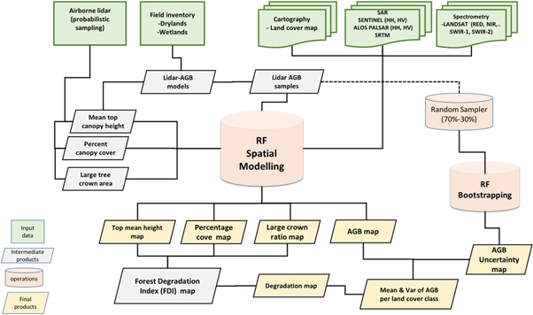
Figure 2. Flowchart showing different components of the methodological system to produce the biomass map of Kalimantan, forest degradation map, and the emission factors for different land use activities in the region. All data used as input to the system are shown in green boxes and include airborne and satellite remote sensing data, land cover and land use map, and ground biomass plots. The intermediate products developed as part of the data processing are shown in grey boxes. Key operations including the development and implementation of spatial modeling and estimation are shown in pink cylinders, and the final products, including the maps, and mean and variance of carbon stocks for land use activities are shown in yellow boxes.
Download figure:
Standard image High-resolution image3. Results
3.1. Lidar-AGB models
The lidar-derived MCH provides strong power-law relationships with AGB for dryland (R2 = 0.81) and wetland forests (R2 = 0.79). The power-law models are significantly different, showing a higher biomass in wetland forests for a given lidar MCH because of a relatively high tree number density and basal area compared with drylands forests (figure 3). We assumed the two models developed in this study capture the largest structural and allometric differences in the region between wetlands and drylands. Without having adequate plots in all forests types present in our study domain, we were not able to verify if there are other vegetation types such as primary swamp pole forests and mangroves with distinct lidar models. Similar assumptions have also been made about the AGB estimates at the ground plots. We assumed that the pan-tropic allometric model provides reasonable estimates of AGB for all forest types in the region (Chave et al 2014).

Figure 3. Lidar-AGB models established as a function of plot-level lidar-derived MCH defined at a resolution of 0.25 ha and 0.1 ha for drylands (green line) and wetlands (blue line), respectively. The percentages of uncertainty are calculated from the ratio of RMSE to the mean AGB. Negative values of bias mean that the model overestimates the observations.
Download figure:
Standard image High-resolution image3.2. Spatial distribution of AGB
The wall-to-wall AGB map of Kalimantan derived from RF algorithm captures the imprints of land use activities and fragmentations on the spatial variations of AGB (table 1 and figure 4). Dense canopy forests with tall trees and high AGB are located inland away from coastal regions and with biomass density increasing at higher elevation where more intact forests are located (figures 4(a) and (b)). The average AGB density of the entire study region from the RF map is 178.4 ± 7.5 Mgha−1, ranging from 34.7 ± 10.1 Mgha−1 for young tree plantations to 312.7 ± 20.6 Mgha−1 for intact lowland forests. The four target land cover classes (denoted with * in table 1) account for 90% of total AGB with an average of 274.1 ± 14.0 Mgha−1.
Table 1. Kalimantan's average AGB density ± the corresponding uncertainty calculated considering the spatial autocorrelation (SI6.4) by land cover type according to the IMF and FDI land cover map (figures 4(b) and (c)). Results are shown for both the lidar sampling and the RF wall-to-wall map. Columns called 5th and 95th correspond to the respective percentiles of the AGB density distribution. The target classes for those we have field data for calibration are denoted with *.
| Surface covered | AGB density (Mgha−1) | 5th (Mgha−1) | 95th (Mgha−1) | |||||
|---|---|---|---|---|---|---|---|---|
| Land cover | lidar (ha) | RF (Mha) | lidar | RF | lidar | RF | lidar | RF |
| Classed derived from IMF land cover map | ||||||||
| Intact lowland forest* | 16 584 | 7.98 | 306.8 ± 1.9 | 312.7 ± 20.6 | 87.4 | 74.9 | 591.2 | 458.8 |
| Intact montane forest* | 765 | 2.26 | 313.8 ± 9.2 | 311.0 ± 51.2 | 175.0 | 233.3 | 458.3 | 387.5 |
| Secondary and degraded forest* | 35 852 | 13.11 | 252.3 ± 1.14 | 261.3 ± 18.0 | 52.83 | 74.5 | 536.86 | 455.6 |
| Peat swamp forest* | 26 511 | 3.62 | 208.2 ± 0.7 | 211.8 ± 12.7 | 70.7 | 30.9 | 357.7 | 403.3 |
| Swamp scrublands | 17 739 | 3.96 | 27.22 ± 0.2 | 40.7 ± 4.9 | 0.17 | 0.5 | 145.60 | 154.1 |
| Scrublands | 9551 | 6.88 | 44.10 ± 0.9 | 54.8 ± 5.5 | 0.1 | 0.9 | 139.1 | 116.0 |
| Tree plantations | 3687 | 7.84 | 88.3 ± 0.7 | 34.7 ± 10.1 | 0.1 | 1.5 | 237.64 | 203.7 |
| Target classes * | 79 710 | 27.0 | 249.6 ± 1.1 | 274.1 ± 14.0 | 62.4 | 71.2 | 508.7 | 448.6 |
| Total | 110 696 | 45.6 | 190.8 ± 0.2 | 178.4 ± 7.5 | 0.8 | 2.6 | 467.6 | 416.4 |
| Classes derived from FDI land cover map | ||||||||
| Intact forest | 13 076 | 7.19 | 386.7 ± 2.3 | 357.2 ± 12.3 | 199.9 | 244.8 | 648.3 | 498.1 |
| Light degraded forest | 6623 | 4.59 | 308.7 ± 2.9 | 320.1 ± 6.4 | 159.5 | 206.7 | 497.6 | 447.4 |
| Moderate degraded forest | 11 655 | 4.96 | 262.3 ± 2.0 | 278.2 ± 11.4 | 106.3 | 149.3 | 444.2 | 407.4 |
| High degraded forest | 5016 | 2.05 | 208.5 ± 2.8 | 222.1 ± 5.3 | 70.9 | 88.1 | 371.6 | 347.0 |
| Severe degraded forest | 12 395 | 3.51 | 138.9 ± 1.4 | 134.2 ± 6.1 | 31.5 | 20.8 | 281.3 | 284.1 |
| Total | 48 765 | 22.3 | 265.0 ± 1.0 | 284.5 ± 11.6 | 64.0 | 77.0 | 524.6 | 452.5 |
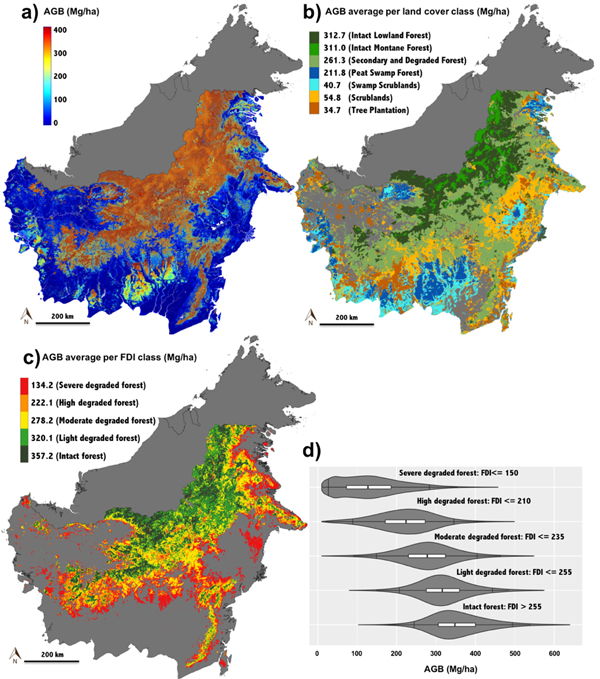
Figure 4. (a) Wall-to-wall AGB density map of Kalimantan and (b) mean density AGB aggregated by land cover class derived from the IMF map (SI2.2). In (c) we show the mean AGB density according to the land cover classes derived from the FDI map (section 2 and SI1.4) and in (d) their distribution through violin plots and box-and-whisker diagrams. The bottom and top of the boxes (commonly called hinges) correspond to the 25th and 75th percentiles and the band inside to the 50th percentile or median. The upper whiskers extend from the hinge to the highest value within the 1.5*IQR of the hinge value, where IQR stands for the inter-quantile range. The vertical lines that cross the whiskers correspond to the 5th and 95th percentile. Outliers are not shown in the graph for visualization purposes.
Download figure:
Standard image High-resolution imageThe estimates of average AGB and uncertainty from the original lidar samples and the RF map are provided in table 2. The AGB of intact lowland (312.7 ± 20.6 Mgha−1) and montane forests (311.0 ± 51.2 Mgha−1) are similar and together they occupy an area nearly as large as the secondary and degraded forests, which stores in average 51 Mgha−1 less than intact forest. The AGB density of peat swamp forests is even lower (211.8 ± 12.7 Mgha−1) but covers a large spectrum of AGB density (the 5th and 95th percentile equal 30.9 and 403.3 Mgha−1). Peatlands are heterogeneous and occupy a highly fragmented landscape ranging from highly dense primary peat swamp pole forest to the stunted peat swamp padang forest with significantly lower AGB. Our result suggests that some of the high biomass forests in Kalimantan are located in the peat swamps surrounding Lake Sentarum and in the Sebangau National Park (dark red areas in the northwest and south of Kalimantan visible in figure 4(a)) that correspond to primary peat swamp tall pole forests (section 3.5). At the same time, the peat swamp forests also show an overall lower AGB due to large-scale degradation and forest fires, particularly in areas outside and surrounding the Sebangau National Park that include large-scale rice fields (Rose et al 2011).
Table 2. Lidar-derived statistics for the main wetlands land cover classes: surface covered, average AGB density ± the corresponding uncertainty calculated considering the spatial autocorrelation (SI6.4), the 5th and 95th percentiles of the distribution. Note that these statistics correspond to the lidar coverage and not to the wall-to-wall RF map. * Peat swamp tall pole forest is also called tall interior forest (Wösten et al 2008).
| Land cover | Surface covered (ha) | Average AGB density (Mg/ha) | 5th | 95th |
|---|---|---|---|---|
| Burnt peat swamp forest | 437 | 18.5 ± 1.3 | 0 | 84.1 |
| Alang-alang | 1113 | 17.8 ± 0.7 | 0 | 54.2 |
| Riverine forest | 1061 | 54.0 ± 1.8 | 0.2 | 163 |
| Peat swamp padang forest | 3422 | 95.5 ± 1.2 | 0.8 | 220.9 |
| Secondary peat swamp tall pole forest* | 26 161 | 207.4 ± 0.7 | 75.4 | 351.9 |
| Primary peat swamp tall pole forest* | 208 | 457.0 ± 13.8 | 119.9 | 900.2 |
Among the remaining vegetation types in Kalimantan, the scrublands cover an area of about 6.88 Mha with average AGB of 54.8 ± 5.5 Mgha−1, and swamp scrublands 3.96 Mha with an average AGB of 40.7 ± 4.9 Mgha−1 (figure 4(b)). Tree plantations cover 7.84 Mha and have an average 34.7 ± 10.1 Mgha−1 indicating that the IMF map only considers the most recent plantations in this class and may have confused older and higher biomass plantations with some remaining natural trees as degraded forests. Note that we assign a higher confidence to the results regarding the target land cover classes because the lidar-AGB models have been developed using field inventory collected over those forest types.
3.3. AGB of degraded forests
The FDI derived degradation map shows a clear gradient of decreasing forest degradation towards inland and mountainous areas (figure 4(c)). The impact of degradation on AGB storage can be estimated using the average density for different FDI classes that range from intact old growth (357.2 ± 12.3 Mgha−1) to severe degraded forests (134.2 ± 6.1 Mgha−1, table 1). The AGB of intact forests increased by about 50 Mg/ha on average after improving the classification of intact and forests using FDI. The AGB distribution shown in violin plots (figure 4(d)) demonstrates a significant overlap among the FDI classes indicating the presence of a large variability of AGB within each class. For instance, intact forest can store low values of AGB on higher elevations and rough topography areas. The intact old growth forests cover the largest area (7.19 Mha), followed by moderate (4.96 Mha) and light (4.59 Mha) degraded forests and with high (2.05 Mha) and severe (3.52 Mha) degraded forests being less abundant.
According to the GIS data layers of logging concessions in Kalimantan (figure SI4), only 20% of the surface covered by secondary and degraded forest class are outside the official logging concession areas. Thus, logging companies are currently managing 22% out of the 27% of Kalimantan's forest biomass stored in secondary and degraded forests. Not surprisingly, the AGB density of forests within the logging concessions (258.0 ± 16.5 Mgha−1) is nearly identical to AGB density in the secondary and degraded forest class (tables 1 and SI3). Other agroforestry classes such as palm oil (9.82 Mha, 59.7 ± 11.3 Mgha−1) and wood fiber (5.5 Mha, 95.4 ± 13.2 Mgha−1) cover large areas and store moderate amounts of AGB. We found the AGB values of forest types in different Kalimantan administrative areas had no significant differences, suggesting that the land use activities and practices are relatively similar across jurisdictions (see SI5.3).
3.4. Lidar versus RF estimates
The difference between lidar- and RF-estimated averaged AGB is relatively low for the target land cover classes, with 1.9% for intact lowland forest, −0.9% for intact montane forest, 3.6% for secondary and degraded forests, and 1. 7% for peat swamp forests (the percentage is relative to average AGB and negative values means that RF underestimates lidar estimates). While that difference is also relatively low regarding the FDI classes (>8%), it reaches 49.5%, 24.3%, and −60.5% for swamp scrublands, scrublands and plantations, respectively (table 1). Nevertheless, these land cover classes account only for the 11% of the total area of Kalimantan and their effects on the average difference between lidar and RF derived AGB for the entire region remain bounded at about 6%.
3.5. AGB in wetland forests
We analyzed the AGB density for the main wetlands present in Kalimantan using AGB estimated directly from the lidar samples (SI4 and table 2). Primary peat swamp tall pole forests (also called tall interior forests, Wösten et al 2008) show a mean AGB density (457.0 ± 13.8 Mgha−1) significantly higher than secondary tall pole forests (207.4 ± 0.7 Mgha−1). These results must be taken with caution because the lidar-AGB model for wetlands does not include plots with AGB exceeding 350 Mgha−1, but the model has been used to predict significantly larger biomass forests. Nevertheless, the AGB map indicates that tall interior forests are within the densest areas of Kalimantan, which agrees with field measurements reported in Verwer and van der Meer 2010 (645.34 Mgha−1). Tall interior forests are highly heterogeneous in terms of forest structure ranging from swamp areas with large tree gaps and low AGB to areas with densely packed and tall trees (5th and 95th percentile in table 2).
Of the remaining wetland vegetation types, peat swamp pandang forest has an AGB density of 95.5 ± 1.2 Mgha−1, because of their short stature and less homogenous cover. Other wetland classes all have low AGB density. The burned peatlands with AGB of 18.5 ± 1.3 Mgha−1 show very little recovery since being classified in the IMF map, and riverine forests, composed largely of woody vegetation, have higher AGB density (54.0 ± 1.8 Mgha−1) than Alang-Alang, which is composed of herbaceous plants.
3.6. Uncertainty analysis
We report the uncertainty in estimating average AGB density for all land cover types and also at jurisdictional scales (table 2, SI3 and SI4) using error propagation throughout the AGB estimation and considering the spatial autocorrelation of the errors (SI6.4). The uncertainty associated with the lidar-AGB models for drylands and wetlands differ significantly (RMSE of 62.2 Mgha−1 and 19.28 Mgha−1, figure 3) due to more heterogeneous nature of dryland structure and degradation compared to wetland forests. Both models showed small bias through cross-validation with plot data with 2.03 Mgha−1 for drylands −1.19 Mgha−1 for wetlands. Similarly, the RF predictions also had small systematic error from cross-validation (bias = 0.49 ± 10.9 Mgha−1) but a relatively large random error (RMSE = 101.9 ± 11.3 Mgha−1) (table SI5).
The uncertainty of the map also remains bounded (<7%) for every land cover class of interest ensuring that the wall-to-wall map provides precise average and total AGB estimates at the scale of land cover classes or jurisdictions. The only exception is the intact montane forests with average AGB of 311 ± 51.2 Mgha−1 and uncertainty that reaches to about 16% (table SI6). For degradation classes derived from FDI thresholds, the uncertainty remains lower (<4%) than similar classes from the IMF map, suggesting that the average AGB of these classes of degradation can be estimated with higher confidence because they are structurally more homogeneous than the IMF map (table 1).
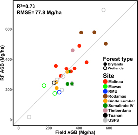
The RF predicted AGB at 1 ha pixels shows a relatively good agreement with an independent set of ground-estimated AGB (R2 = 0.73, figure 5). The field plots used for comparison have been covered by airborne lidar but were not used for the development of lidar-AGB models (SI6.5). However, these results should be taken with caution because the plots are located within the lidar flights and the RF predictions are prone to overfitting the lidar data used in training the map. Field plots located in areas with forest structure significantly different from those covered by the lidar may have larger uncertainty.
Figure 5. Comparison between field-derived AGB and the estimates of our map. Smaller fields plots have been aggregated to 1 ha in order to compare to the AGB map (refer to SI6.5).
Download figure:
Standard image High-resolution image
4. Discussion and conclusions
4.1. Lidar and ground sampling design
The derived AGB distribution in Kalimantan forests is based on a probabilistic airborne lidar sampling that ensures unbiased estimates of mean and total forest AGB subject to the choice of the lidar-AGB model (Ståhl et al 2016), similar to ground inventory sample measurements that can produce unbiased estimates given the right biomass allometry. However, due to requirements for planning airborne flights in the region, the lidar sampling design provided only 29 lidar scenes for a total of 29 000 ha. These samples, although randomly located across the region, are not widespread and do not adequately capture the variations of all types of forests. Selecting smaller sampling areas (∼500 ha) and a larger number of samples could have improved the RF predictions and the uncertainty of estimates for all forest types present in the region. Given additional resources, an improved sampling strategy based on land cover stratification can be used for future sampling design.
We collected a larger number of airborne lidar data over existing plot networks to allow development of reliable and unbiased lidar-AGB models. The lack of any systematic inventory plots in the region and the diversity in existing plot size and quality are considered sources of errors that cannot be readily quantified or mitigated. However, our methodology allows for improvement of lidar-AGB models by acquiring additional ground inventory data within the lidar coverage.
4.2. Spatial uncertainty
Unlike the previous AGB maps (Saatchi et al 2011a, Baccini et al 2012), we developed forest-type specific lidar-AGB models (for drylands and wetlands) that adjust to differences in the 3D forest structure and tree density in order to reduce the uncertainty associated with lidar estimates of AGB. The average AGB values for the target land cover classes derived from the RF prediction map are in agreement with the lidar-derived estimates, suggesting the map as a reliable tool to estimate the average AGB density for different land cover classes or at landscape scales (100–10 000 ha). One of the limitations of the RF prediction algorithm is the problem of overfitting the distribution that may lead to underestimation of the range of biomass variability, a so-called dilution bias. Although we included a bias correction approach that improves the uncertainty of the RF prediction bias (Xu et al 2016), the map still shows differences at the 5th and 95th percentiles with the lidar-AGB distribution (table 1).
Furthermore, the map may slightly underestimate high biomass density due to the lack of sensitivity of satellite imagery used in RF models. Upcoming satellite missions (NASA-ISRO NISAR mission, NASA GEDI mission and ESA BIOMASS mission) are expected to improve the sensitivity of measurements to forest structure and AGB across the entire biomass range, particularly in the dense tropical forests and across the complex terrains (LeToan et al 2011, Yu and Saatchi 2016). However, the underestimation is in general much smaller than the predicted sensitivity of the satellite data used as input layers to develop the machine learning algorithms. Both the existing radar and optical sensors are known to be saturated over dense tropical forests when used directly in parameteric models to estimate forest biomass (Saatchi et al 2011b). The non-parametric machine-learning approach has a significantly more efficient way of using the spatial variations of the data layers to extrapolate or estimate forest biomass from the training data. The approach includes the use of spatial distribution of training data from lidar-derived biomass to increase the probability of predicting biomass values across landscapes. For example, most remaining high biomass forests are located across upland and higher elevation landscapes and the RF model uses the SRTM (elevation and surface ruggedness) to predict the high biomass forests in Kalimantan (S13). In addition, other layers such as short wavelength and near infrared bands of multi-spectral Landsat imagery potential help to separate high biomass forests due to shadows from dense layered canopy structures and older aged leaves from open and younger aged leaves of degraded and secondary forests (Steininger 1996).
4.3. Intact forests versus majestic forests
The average AGB estimates for drylands intact forests reported in the literature in recent years are relatively higher (436 Mgha−1 in Slik et al 2010, 426 Mgha−1 in Qie et al 2017) than the estimates from the RF map (357.2 Mgha−1) or lidar sampling (386.7 Mgha−1). Similarly, the RF AGB prediction of the peat swamp forests of 218 ± 12.7 Mgha−1 is relatively lower than those published by Verwer and van der Meer (2010) of 278.85 Mgha−1 and, Murdiyarso et al (2010) of 269.55 Mgha−1. We expect our results from either the RF map or the lidar sampling to be more realistic because of the probabilistic sampling approach used in our study. Most research plots in these studies do not follow a systematic sampling and are often located in areas of high biomass forests that lead to an overestimation of the AGB in Kalimantan, the so-called majestic forest effect (Sheil 1995). The high-resolution lidar observations used in our study capture the natural variability of structure and biomass in intact forests caused by topography, soil variations, wind and other natural disturbance. By providing the 5th and 95th biomass values for different forest types, the range of biomass in intact forests can be readily compared with published results. Furthermore, by adjusting the values of mean canopy height and percent of large trees, the spatial products from this study can be used to delineate areas of high biomass density characteristic of the majestic forests.
4.4. Logging versus degradation
Following the CDM of the Kyoto Protocol guidelines (UNFCCC 2002), we define forest as an area with vegetation higher than 5 m and with cover that exceeds 30% of the 1 ha grid cells. We developed the FDI to map different degrees of forest degradation and improve the IMF based on Landsat imagery. The average biomass loss from degradation based on our study is much larger (up to 50%) than what is reported in the literature for selectively logged forests in Kalimantan (3%–15%) (Sasaki and Putz 2009, Kronseder et al 2012, Pearson et al 2014). Using the FDI index, we were able to delineate the lightly and moderately degraded forests within the Landsat land cover map that closely capture the selectively logged forests. However, other types of degradations due to different logging intensity (Pearson et al 2014), fragmentations, loss of biomass from edge effects, and fire, reported from our study, must be considered as degradation in accounting for carbon loss and emissions in the region.
4.5. Carbon storage versus potential
Based on the RF map, the intact and light degraded forests cover (11.78 Mha) approximately the same size area of moderate to severe degraded forests combined (10.53 Mha), suggesting a large area of dryland forests with significant potential for carbon sequestration. By focusing on dryland forests, the total carbon stored in about 22.3 Mha of forests is approximately 3.1 PgC (using average AGB of 284.5 Mgha−1 from table 1, and the carbon fraction of 0.48). The emission factors associated with degradation can be calculated by the difference between the average carbon storage of intact and degraded forests that multiplied by the area occupied by the degraded forests provide the carbon sequestration or storage potential of degraded forests. We find the storage potential of degraded forests to be about 0.8–1.1 PgC depending on emission factors calculated from lidar or RF map. Kalimantan degraded forests have significantly larger storage potential per ha (70.2 MgCha−1) than the entire Latin America second-growth forests of age 1 to 60 years (35.33 MgCha−1) and over a shorter period of time (Chazdon et al 2016).
Acknowledgments
The research was carried as part of NASA's Carbon Monitoring System at the Jet Propulsion Laboratory, California Institute of Technology, under a contract with the National Aeronautics and Space Administration. Support for the larger team was provided via NASA Grant #NNX13AP88G. Support for Jerome Chave's contribution was by 'Investissement d'Avenir' grants managed by Agence Nationale de la Recherche (CEBA, ref. ANR-10-LABX-25-01 and TULIP, ref. ANR-10-LABX-0041).
We are grateful for receiving field plot data generously provided by several research groups, including—Shijo Joseph and the Center for International Forestry Research (CIFOR) in Bogor, Indonesia; the Kalimantan Forest and Climate Partnership (KFCP); Dr Matthew Warren; Rezal Kusumaatmadja and Rimba Makmur Utama; and Winrock International.