the Creative Commons Attribution 3.0 License.
the Creative Commons Attribution 3.0 License.
Seasonal streamflow forecasts for Europe – Part I: Hindcast verification with pseudo- and real observations
Wouter Greuell
Wietse H. P. Franssen
Hester Biemans
Ronald W. A. Hutjes
Seasonal predictions of river flow can be exploited among others to optimise hydropower energy generation, navigability of rivers and irrigation management to decrease crop yield losses. This paper is the first of two papers dealing with a physical model-based system built to produce probabilistic seasonal hydrological forecasts, applied here to Europe. This paper presents the development of the system and the evaluation of its skill. The variable infiltration capacity (VIC) hydrological model is forced with bias-corrected output of ECMWF's seasonal forecast system 4. For the assessment of skill, we analysed hindcasts (1981–2010) against a reference run, in which VIC was forced by gridded meteorological observations. The reference run was also used to generate initial hydrological conditions for the hindcasts.
The skill in run-off and discharge hindcasts is analysed with monthly temporal resolution, up to 7 months of lead time, for the entire annual cycle. Using the reference run output as pseudo-observations and taking the correlation coefficient as metric, hot spots of significant theoretical skill in discharge and run-off were identified in Fennoscandia (from January to October), the southern part of the Mediterranean (from June to August), Poland, northern Germany, Romania and Bulgaria (mainly from November to January), western France (from December to May) and the eastern side of Great Britain (January to April). Generally, the skill decreases with increasing lead time, except in spring in regions with snow-rich winters. In some areas some skill persists even at the longest lead times (7 months).
Theoretical skill was compared to actual skill as determined with real discharge observations from 747 stations. Actual skill is generally substantially less than theoretical skill. This effect is stronger for small basins than for large basins. Qualitatively, the use of different skill metrics (correlation coefficient; relative operating characteristics, ROC, area; and ranked probability skill score, RPSS) leads to broadly similar spatio-temporal patterns of skill, but the level of skill decreases, and the area of skill shrinks, in the following order: correlation coefficient; ROC area below-normal (BN) tercile; ROC area above-normal (AN) tercile; ranked probability skill score; and, finally, ROC near-normal (NN) tercile.
- Article
(10015 KB) - Full-text XML
- Companion paper
-
Supplement
(4085 KB) - BibTeX
- EndNote


Society may benefit from seasonal hydrological forecasts, i.e. hydrological forecasts for future time periods from more than 2 weeks up to about 1 year (Doblas-Reyes et al., 2013). Such predictions can, for example, be exploited to optimise hydropower energy generation (Hamlet et al., 2002), navigability of rivers in low-flow conditions (Li et al., 2008) and irrigation management (Ghile and Schulze, 2008; Mushtaq et al., 2012) to decrease crop yield losses. In order to be of any value in decision-making processes in such sectors, forecasts must be credible, i.e. be skilful in predicting anomalous system states, in addition to being relevant to the decision-making process and acceptable for the user (e.g. Bruno Soares and Dessai, 2016). In this paper we will introduce WUSHP (Wageningen University Seamless Hydrological Prediction system), a dynamical, model-based system (see Yuan et al., 2015) that was built around the variable infiltration capacity (VIC) hydrological model and ECMWF's seasonal forecast system 4, to produce seasonal hydrological forecasts. It will be applied to Europe. The usefulness of the system depends partially on the level of its skill and the paper will therefore focus on an extensive assessment of the skill of WUSHP. The usual method of assessing skill of predictive systems is by analysing hindcasts, a strategy that will be adopted here as well.
During recent years, a number of systems for making seasonal hydrological forecasts have been developed. Examples are the University of Washington's surface water monitor (SWM; Wood and Lettenmaier, 2006) and the African drought monitor (Sheffield et al., 2014). Seasonal hydrological forecasting systems for the entire continent of Europe are scarce (Bierkens and van Beek, 2009; Thober et al., 2015), but a few more concentrate on smaller domains such as the British Isles (Svensson et al., 2015), Iberia (Trigo, 2004) or France (Céron et al., 2010; Singla et al., 2012).
Thober et al. (2015) forced a mesoscale hydrological model with meteorological hindcasts from the North American Multi-Model Ensemble (NMME) to investigate the predictability of soil moisture in continental Europe, excluding Fennoscandia. Evaluating at seasonal resolution a number of forecasting techniques that produced distinct variations in the magnitude of skill, they found that spatial patterns in skill were remarkably similar among the different techniques, as well as comparable to the spatial patterns of the autocorrelation (persistence) of reference soil moisture. High skill was found in eastern Germany and Poland, Romania, the southern Balkans and eastern Ukraine as well as northwestern France. Less skill was found in the mountainous areas of the Alps and the Pyrenees, the northern Adriatic and Atlantic coast of the Iberian Peninsula. Most skill was found for winter months (DJF) and the least for autumn (SON), with this minimum shifting to summer (JJA) at long lead times (6 months).
Bierkens and van Beek (2009) developed an analogue events method to select annual ERA40 meteorological forcing on the basis of annual SST anomalies in the northern Atlantic and then made hydrological forecasts with a global-scale hydrological model applied to Europe. Evaluating only skill for winter and summer half-year mean discharge, they found wintertime skill in large parts of Europe with maxima in eastern Spain and in a zone beginning in the southern Balkans and Romania, running through eastern Poland and western Russia, and ending in the Baltic states and Finland. Summertime skill was lower, generally by about 50 % and even more around the Alps and the Adriatic. A climate forecast based on the North Atlantic Oscillation (NAO) added significant skill only in limited areas, such as Scandinavia, the Iberian Peninsula, the Balkans and around the Black Sea.
Svensson et al. (2015) found skilful winter river flow forecasts across the whole of the UK due to a combination of skilful winter rainfall forecasts for the north and west and a strong persistence of initial hydrological conditions in the south and east. Strong statistical correlations between the NAO index and winter precipitation in Iberia lead to skilful forecasts of JFM river flow and hydropower production (Trigo et al., 2004). Céron et al. (2010) and Singla et al. (2012) set up a high-resolution river flow forecasting system (8 km) over France, for which the seasonal climate forecast improved the MAM skill over northern France, but worsened it over southern France (compared to a river flow model with proper initialisation of soil moisture, snow, etc., but random atmospheric forcing). Demirel et al. (2015) found that both two physical models and one neural network over-predict run-off during low-flow periods using ensemble seasonal meteorological forcing for the Moselle basin. As a result forecasts of more extreme low flows are less reliable than forecasts of more moderate ones.
It is quite common in seasonal hydrological forecasting (e.g. Shukla and Lettenmaier, 2011; Singla et al., 2012; Mo and Lettenmaier, 2014; and Thober et al., 2015) but also in medium range forecasting (i.e. 14 days in Alfieri et al., 2014) to determine prediction skill by comparing the hindcasts with the output from a reference simulation. A reference simulation is a simulation made with the same hydrological model as the hindcasts, except that the forcing is taken from meteorological observations or from a gridded version of meteorological observations. The reference simulation can best be regarded as a simulation that attempts to make a best estimate of the true conditions (for instance, in terms of discharge, soil moisture and evapotranspiration), using the modelling system. We will refer to the output of such a reference simulation as pseudo-observations (alternatively named “true discharge” in Bierkens and Van Beek, 2009, “synthetic truth” in Shukla and Lettenmaier, 2011, “reanalysis” in Singla et al., 2012, and “a posteriori estimates” in Shukla et al., 2014). We prefer the term “pseudo-observations” over “reanalysis” since the latter has a meteorological connotation that often implies the use of some form of (variational) data assimilation. We did not attempt any form of assimilating observed hydrological variables, such as discharge, in our reference run.
Pseudo-observations have the important advantages of being complete in the spatial and the temporal domain and being available for all model variables. Also, they are suitable for the quantification of small sensitivities, e.g. to bias correction of the meteorological forcing, which would be hard to detect with real observations. Finally, assessment of skill based on pseudo-observations reduces model errors from the analysis to a minimum, which is especially useful when addressing various sources of skill (Wood et al., 2016), something we will do in the companion paper (Greuell et al., 2016).
The downside of pseudo-observations is, of course, that they are not equal to real observations. In this paper we will determine the performance of the prediction system not only with pseudo-observations, but also with real observations of discharge (like e.g. Koster et al., 2010 and Yuan et al., 2013) and compare the skill found with the two different approaches (theoretical and actual skill, according to Van Dijk et al., 2013). Such a comparison was previously made by Bierkens and Van Beek (2009) and Van Dijk et al. (2013) and they found that theoretical skill generally exceeds actual skill. This is in line with the fact that the pseudo-observations are obtained with the same model as the hindcasts, which should logically lead to an overestimation of the skill when the pseudo-observations are used for verification. We thus hypothesise that theoretical skill exceeds actual skill. In this paper we will not only analyse the difference between the skills obtained with the two different types of data but also discuss in some detail conceptual differences between using pseudo- and real observations for verification.
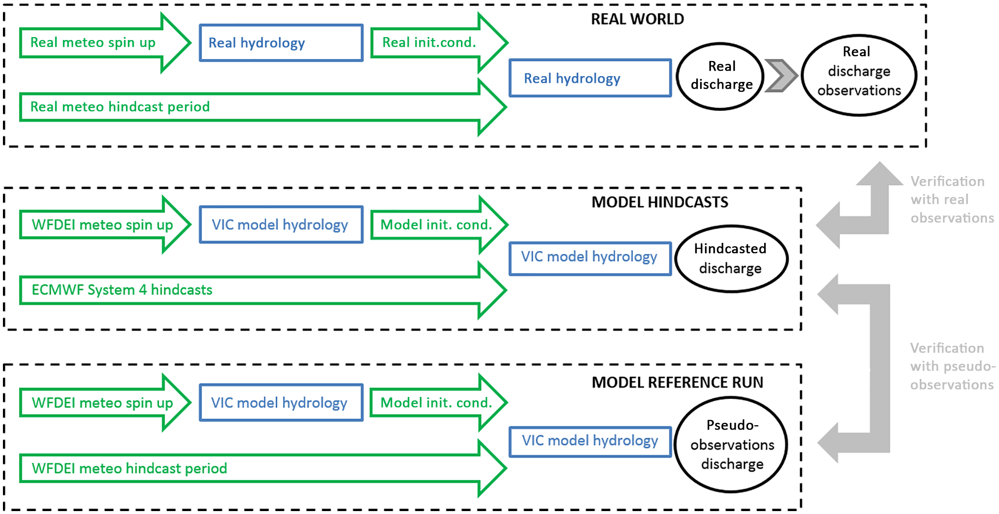
Figure 1Set-up of the present study. The lower two dashed boxes summarise the set-up of the forecast system itself. The upper dashed box represents the real world. The filled arrows on the right-hand side represent verification of hindcasts (in the middle) with pseudo-observations (bottom) and with observations of real discharge (top). In each box the flow at the upper left represents the creation of initial conditions while the flow below that (a single arrow) represents the meteorological forcing.
This paper aims to analyse to what extent WUSHP is able to predict run-off and discharge in Europe over the full annual cycle and for lead times up to 7 months. We aim to assess skill at monthly resolution instead of seasonal or semi-annual aggregates. Where many studies use the correlation coefficient as a main skill metric we will also assess skill using two probabilistic metrics, namely ROC (relative operating characteristics) area and RPSS (ranked probability skill score; see Sect. 2.3). The second aim of the paper is to get a better understanding of the effects of using pseudo-observations, as opposed to using actual observations, for the verification of hindcasts. In the next section we describe the concept and details of our modelling (Sect. 2.1) and analysis approach (Sects. 2.2 and 2.3). We will start the result section by assessing theoretical skill of the run-off hindcasts (Sect. 3.1) and then proceed to theoretical skill of the discharge hindcasts and a comparison between theoretical skill of discharge and run-off in Sect. 3.2. Differences between theoretical and actual skill of discharge will be presented (Sect. 3.3) followed by an analysis of differences in skill determined with various metrics in Sect. 3.4. The discussion starts with a conceptual analysis of reasons for differences in actual and theoretical skill (Sect. 4.1), followed by a discussion of uncertainties (Sect. 4.2) and implications (Sect. 4.3).
In a companion paper (Greuell et al., 2016) we analyse the reasons for the presence or lack of skill discussed in the present paper, using two different methods. Firstly, skill in the forcing and other directly related hydrological variables, such as evapotranspiration, are analysed. Secondly, a number of experiments similar to the conventional ensemble streamflow prediction (ESP) and reverse-ESP experiments, which isolate different causes of predictability, are discussed. In the results and discussion sections of the present paper we will occasionally look forward to the identified causes of skill.
In the following subsections we will describe the various components of WUSHP (2.1), the real discharge observations (2.2) and the methods of analysis (2.3). Figure 1 provides an outline of the system, which consists of the hindcasts themselves (middle box in the figure) and a model reference run (lower box). The hindcasts will be verified by means of the pseudo-observations, which are generated by the reference simulations, and by real discharge observations, which are “generated” in the real world (upper box). Differences between these two types of verifications will be discussed in Sect. 4.1.
2.1 The model, workflow and forcing data for the hindcasts and the reference simulation
WUSHP consists of two simulation branches: a single reference simulation (lower box in Fig. 1) and the hindcasts themselves (middle box in same figure). In both branches, terrestrial hydrology is simulated with the variable infiltration capacity model (VIC, see Liang et al., 1994), which runs on a domain extending from 25∘ W to 40∘ E and from 35 to 72∘ N, including 5200 land-based cells of 0.5∘ × 0.5∘ (see maps in e.g. Fig. 2). VIC is forced by a gridded data set of daily meteorological data (7 variables: precipitation, minimum and maximum temperature, atmospheric humidity, wind speed, and incoming short- and long wave radiation).
In the reference simulation VIC is forced by the WATCH Forcing Data ERA-Interim (WFDEI; Weedon et al., 2014) for the period of 1979–2010, of which the first 2 years were used to spin up the states of snow, soil moisture and discharge and were not used in further analysis. The reference simulation has the dual aim to create the pseudo-observations for verification purposes (lower box in Fig. 1) and to create a best estimate of the temporally varying model state, which is then used for the initialisation of the hindcasts (flow from the upper left in the middle box of Fig. 1).
The second branch, the hindcasts, consists of three steps. Seasonal predictions of the same set of 7 meteorological variables (see above) are taken from ECMWF's seasonal forecast system 4 (S4 hereafter) at daily resolution. These are then bias corrected using WFDEI as the reference data set. Finally, VIC is run with the bias-corrected S4 hindcasts as forcing, taking initial states from the reference simulation.
The S4 hindcasts used in the present study include 15 members, cover the period from 1981 to 2010 and consist of simulations with a duration of 7 months, starting and initialised on the first day of every month (see Molteni et al., 2011, and the ECMWF seasonal forecast user guide, online). The S4 ensemble is constructed by combining a five-member ensemble analysis of the ocean initial state with SST perturbations of that state and with activation of stochastic physics.
All seven meteorological forcing variables were regridded with bilinear interpolation from the 0.75 × 0.75∘ latitude and longitude grid of the S4 hindcasts to a 0.5 × 0.5∘ grid. Since bias correction generally improves forecasting skill, the quantile mapping method of Themeßl et al. (2011) was applied to bias-correct the forcing variables, taking the WFDEI as reference. For each variable and grid cell, 84 correction functions were established and applied by separating the data according to target month (12) and lead month (7). Such empirical distribution mapping of daily values has been successful in improving especially forecast reliability (rather than sharpness and accuracy; Crochemore et al., 2016).
VIC was run for the period of the S4 hindcasts (1981–2010). Additionally, for the reference simulation 2 extra years (1979–1980) were simulated to spin up the states of snow, soil moisture and discharge. The hindcast simulations were initialised with states of soil moisture and snow from the reference simulation, so for these variables spin up was not needed. However, due to the set-up of the routing module of VIC, the state of discharge could not be saved and loaded. Hence, to spin up discharge, each 7-month hindcast simulation was preceded by a 1-month simulation with WFDEI forcing. Since the hindcasts cover 30 years with 12 initialisation dates each and consist of 15 members, a total of 5400 hindcast simulations was carried out.
VIC is run in so-called “energy balance mode”, which requires resolving the diurnal cycle. Therefore, internally the model temporally disaggregates the daily input to 3-hourly data and runs with a time step of 3 h. The output of all variables is again at a daily resolution. Because snow may contribute significantly to the seasonal predictability of other hydrological variables, VIC was run with the option of subgrid elevation bands. This means that for each grid cell, calculations were carried out at up to 16 different elevations, with the aim of simulating the elevation gradient of snow. VIC was run in natural flow mode, i.e. river regulation, irrigation and other anthropogenic influences were not considered.
Simulations of historic discharge made with VIC (and four other hydrological models) were validated with observations from large European rivers by Greuell et al. (2015) and Roudier et al. (2016). VIC exhibits a fairly small average bias (across 46 stations) of +23 mm yr−1 (=7 %) and overall differentiates well between low and high specific discharge basins with a spatial correlation coefficient of 0.955. However, specific discharge is overestimated in the Mediterranean and underestimated in northern Fennoscandia. Annual cycles are fairly well reproduced across Europe, though VIC somewhat overestimates their amplitude. In northern Fennoscandia the spring peak is too late and lasts too long. Annual cycles are best reproduced for rain-fed rivers in central Europe, while those for rivers with significant snow dynamics are good (Alps). However, the annual cycle is more poorly reproduced in basins with strong soil freezing dynamics (northern Fennoscandia) or strong damping of discharge amplitudes by large lakes (southern Finland).
Perhaps more relevant in the present context is the model's capability to reproduce inter-annual variations in discharge. On average across 22 discharge stations, the standard deviation of simulated annual discharge was 9 % higher than observed and the spatial correlation coefficient between the two was 0.94. Like most models, VIC is better in simulating high flows (95 percentile: Q95) than low flows (Q5); the first is slightly overestimated and the second more seriously underestimated. The inter-annual variation in Q5 is overestimated in central Europe and the Alps, but underestimated in Fennoscandia (overall spatial correlation coefficient across Europe 0.40). The inter-annual variation in Q95 shows no clear spatial pattern and the overall spatial correlation coefficient is 0.70.
All validation results discussed in these two paragraphs are for the VIC model forced by E-OBS (v9, Haylock et al., 2008). Our forcing, WFDEI, shows higher precipitation (+104 mm yr−1) across most of Europe, except for the Alps, Scotland and westernmost Norway. According to Greuell et al. (2015) this leads to higher mean discharge, higher inter annual variability and higher Q95 (but not Q5) of simulated discharge for almost all stations.
2.2 Discharge observations
For the assessment of skill with real discharge observations, two data sets with daily resolution were acquired from the Global Runoff Data Centre, 56068 Koblenz, Germany (GRDC): the GRDC data set and the European Water Archive (EWA) data set. We mapped these two station data sets onto the VIC grid with its resolution of 0.5∘ × 0.5∘ and aggregated the daily data at a time step of a month. To enable the investigation of the effect of basin size on some of our results, we made two subclasses of observations. The first comprised observations for basins larger than 9900 km2 (called large basins hereafter) and the second contained basins smaller than the area of the grid cells, i.e. smaller than about 2530 km2 in southern Europe (at 35∘ N) and 1050 km2 at 70∘ N (called smaller basins hereafter).
Initially, in many cases the location of observation stations did not match with the corresponding river in the digital river network used in the routing calculations (DDM30, see Döll and Lehner, 2002). We corrected for this issue by matching the observations with the simulations by means of basin size. The size of the model basins (called model basin area hereafter) was determined by the DDM30 network. The size of the basins upstream of the observation stations (called station basin area hereafter) was taken from the metadata of the observations. First the station basin area was compared to the model basin area of the cell that is nearest to the station (called nearest model cell basin area hereafter). After this first step the mapping procedure for each observation differed between the two classes of basins.
For large basins we proceeded as follows:
-
If the station and the nearest model cell basin area differed by less than 15%, the observations were matched with the model calculations for the nearest model cell.
-
Otherwise, the station basin area was compared with the model basin area of the eight cells surrounding the nearest model cell.
-
The minimum of the eight differences was determined.
-
If that minimum was less than 15%, the simulations for the corresponding cell were matched with the observations.
-
Otherwise, the station was discarded.
For small basins we proceeded as follows:
-
If the nearest model cell did not have an influx from any of the neighbouring cells, its simulations were matched with the observations.
-
Otherwise, all of the eight neighbouring cells without influx were selected.
-
Their simulations were averaged and matched with the observations.
We further discarded all observations with less than 21 years of data within the simulation period (1981–2010) for any of the months of the year. The final data set within our European domain contained 111 cells with observations for large basins and 636 cells with observations for basins smaller than a model grid cell.
These data sets do not include any variable or parameter characterising the level of human impact. To enable analysis of the effect of anthropogenic flow modifications on predictive skill, we quantified the human impact by performing two model simulations with the Lund–Potsdam–Jena managed Land (LPJmL) model (Rost et al., 2008; Schaphoff et al., 2013). This model was operated at the same spatial resolution (0.5∘ × 0.5∘) and with the same river network (DDM30) as VIC, but LPJmL does include dams (GRanD database; Lehner et al;. 2011) and associated reservoir management. From the discharge output of a natural LPJmL run and an LPJmL run with reservoir operation and irrigation, the human impact at cell level was quantified by computing the so-called amended annual proportional flow deviator (AAPFD; see Marchant and Hehir, 2002). For the analysis in Sect. 3.3, we selected all discharge observations for large basins with an AAPFD <0.3, i.e. basins with a relatively small degree of human impact (about half of all 111 basins).
2.3 Methods of analysis
From the model output, consisting of daily means, monthly mean values were computed, which were then used for the analysis. The analysis is restricted to run-off, defined here as the amount of water leaving the model soil either along the surface or at the bottom, and discharge, defined here as the flow of water through the largest river in each grid cell. Discharge accumulates all run-off from cells that are upstream in the model river network, with delays due to transport inside cells and through the river network. Hence, whereas run-off represents only local hydrological processes, discharge aggregates hydrological processes occurring in the entire basin upstream of a particular cell.
Instead of analysing skill per target season and/or for a number of consecutive lead months, we analysed skill for every combination of the 12 target and the 7 lead months. The thus achieved higher temporal resolution of the skill metrics enables a more accurate determination of the beginning and end of periods of skill. Moreover, skill at a monthly resolution provides the possibility to determine the consistency of the skill where we define consistent skill as skill that persists during at least two consecutive target or lead months. In accordance with Hagedorn et al. (2005) we designated the first month of the hindcasts as lead month zero, so target month number is equal to the number of the month of initialisation plus the lead month number.
Three skill metrics (see Mason and Stephensen, 2008, for a good discussion of the why and how of these) were computed for each target and lead month separately: (i) the correlation coefficient between the observations and the median values of the hindcasts (referred to as the correlation coefficient or R), (ii) the area beneath the relative operating characteristics curve (ROC area) and (iii) the ranked probability skill score. The ROC area is computed for three categories of the observations and hindcasts with an equal number of values, namely the categories containing the one-third highest, lowest and the remaining values (upper, lower and middle tercile, respectively; above-, below- and near-normal – AN, BN and NN – categories). The same subdivision of observations and hindcasts in terciles was made to compute the RPSS. Since none of these metrics is sensitive to systematic biases in the forecasting system, no attempt was made to correct simulated run-off or discharge for any such errors prior to computing the skill metrics. So we focus our evaluation on the models' capability to predict river flow anomalies rather than absolute river flows.
All three skill metrics quantify, though in different ways, how well the ranking of the hindcasts matches the ranking of the observations. The correlation coefficient is a measure of the association between (pseudo-) observation and forecast ensemble median; we used the Pearson correlation coefficient. The ROC area is a measure of resolution or discrimination and indicates whether the forecast probability of an event (i.e. value falling in the considered tercile) is higher when such an event occurs compared to when not. The RPSS is a measure of accuracy and summarises in a single number the skill of a forecast system to make forecasts with the correct percentage of ensemble members falling in any of the defined terciles. Perfect forecasts have values of 1 for all three skill metrics. Climatological forecasts (probabilistic forecasts that in our case each year predict a 1/3 chance of a high or low anomaly occurring) lead to values of 0 for R, 0.5 for the ROC area and 0 for the RPSS. In the computation of significance of the RPSS, sampling errors, i.e. the limited number of ensemble members, constitute a problem. They cause a bias in the RPSS when climatology is used as reference (Mason and Stephenson, 2008). Therefore, the reference for the calculation of the RPSS was generated by sampling randomly from the multinomial distribution with and N=15 (the number of ensemble members). In the present paper each metric is designated as significant for p values less than 0.05. For a data set of 30 years, this implies R is significant for values >0.31, ROC area for values >0.69 and RPSS for values that vary depending on the outcome of the random draw for the reference. We checked these procedures to determine significance by analysing hindcasts that have no skill. Such hindcasts indeed produced for all metrics a fraction of cells with significant skill near the expected value of 0.05 (the p value), indicating that the procedures are correct.
To a large extent, we found that our results and conclusions, in terms of spatio temporal patterns of skill, are independent of the chosen metric. Hence, and because among the three metrics the correlation coefficient is the easiest to understand, we will discuss results mostly in terms of the correlation coefficient, which is in line with Doblas-Reyes et al. (2013). The sensitivity to the chosen metric and significant differences between these metrics will be discussed in Sect. 4.2.
All metrics were computed using the low- and high-level R packages SpecsVerification (Siegert et al., 2014) and easyVerification (Bhend et al., 2016), respectively. Metrics cannot be computed (because they become ill-defined) if observations or hindcasts within the entire 30-year period consist of more than one-third zeros or one-sixth ties (i.e. equal values). Such skill gaps (i.e. the white terrestrial cells in Figs. 2 and 3) mainly occur in the far north due to rivers that are frozen for at least a month in winter.
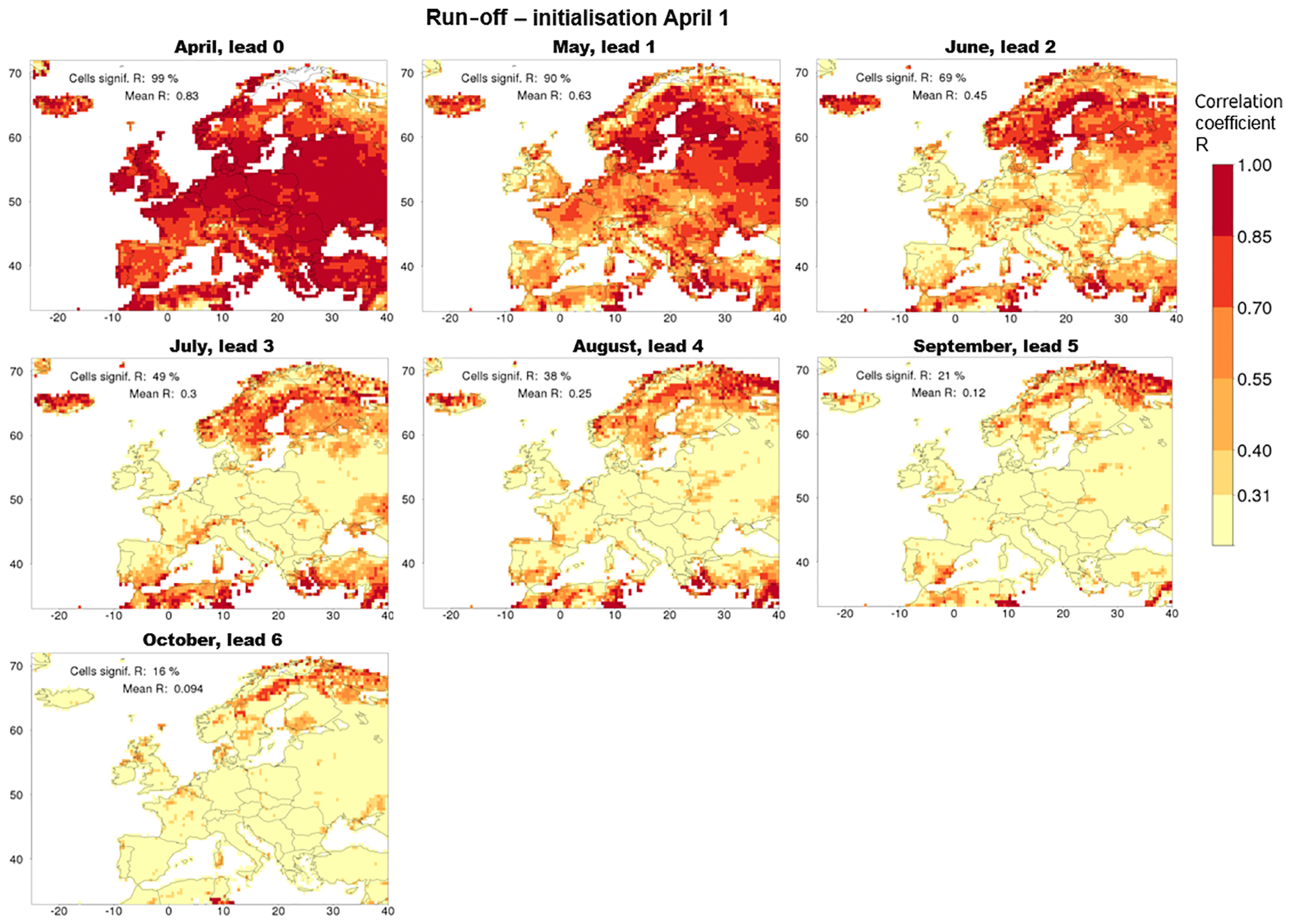
Figure 2The skill of the run-off hindcasts initialised on 1 April for all 7 lead months. The skill is measured in terms of the Pearson correlation coefficient between the median of the hindcasts and the observations (R). The threshold of significant skill lies at 0.31, so yellow cells have insignificant skill while darker cells have significant skill. White, terrestrial cells correspond to cells where observations or hindcasts consist of more than one-third zeros or one-sixth ties. The legend provides the fraction of cells with significant values of R (at the 5 % level) and the domain-averaged value of R.

Figure 3Annual cycle of skill (R) of run-off hindcasts for 12 target months, initialised at the beginning of the second month before (lead month 2). More explanation is given in the caption of Fig. 2.
3.1 Spatio-temporal variation of skill in run-off forecasts
A total of 84 maps of the skill of the run-off hindcasts were produced for all 12 initialisation months and all 7 lead months (all are presented in the Supplement Fig. S1). Two cross-cuts through that collection are shown in Fig. 2 (for a single initialisation month) and Fig. 3 (for a single lead month). The seven panels of Fig. 2 show the skill of the hindcasts initialised on 1 April as a function of lead time. Cells with an insignificant amount of skill are tinted yellow; cells where no metric could be computed remain white. In lead month 0, significant skill is found across almost the entire domain (99 % of the cells). After the first lead month, the fraction of cells with significant skill gradually decreases to reach 16 % at the longest lead time (lead month 6). This is more than expected for the case of completely unskilful simulations (5 % of the cells), so at the end of the hindcast simulations significant skill that does not occur due to chance is still present in some regions. The general impression is that the pattern of skill does not move in space but that skill is fading, i.e. for individual grid cells R is mostly decreasing with increasing lead time. The same holds for initialisation in other months (see Fig. S1 in the Supplement), with important exceptions better identified with Fig. 5 and discussed there.
The 12 panels of Fig. 3 show the annual cycle of the skill of the hindcasts for lead month 2, which is selected (also in Figs. 6, 7 and 9) because at that lead time approximately 50 % of the cells have significant skill. Consistent skill (persistent during at least 2 consecutive target months) is found in the following regions (causes of skill are reproduced here from the companion paper, Greuell et al., 2016):
-
Fennoscandia. Much skill is present during the entire year, except for target months November and December, and there is a dip in the skill in April. Most of the skill is due to initial conditions of soil moisture. On average across the entire region, the skill reaches a maximum in May and June, i.e. at the end of the melting season, which is, as shown in the companion paper, largely due to initialising snow. Compared to the rest of the peninsula, there is generally less skill along the Scandinavian mountain range. The companion paper shows some evidence that this may be due to high variability of orographic rain, ill-represented in the S4 hindcasts.
-
Poland and northern Germany. The core period lasts from November to January, but it is extended with periods of less skill into October and the months from February to May. Here the initialisation of soil moisture is the dominant cause of skill. Snow initialisation contributes in April and May.
-
Western France, more or less from Paris to Brittany and roughly from December to May. Skill derives from the initialisation of soil moisture.
-
The eastern side of Great Britain from January to April. Also here the skill derives from soil moisture initialisation.
-
Romania and Bulgaria. The core and the whole period are the same as that for Poland and northern Germany.
-
The southern part of the Mediterranean region from June to August. The high amounts of skill are limited to the coastal parts of northern Africa, Sicily, southern Greece, Turkey, Syria and Lebanon. This skill is due to initialisation of soil moisture.
-
The Iberian peninsula in March and August with smaller amounts of skill in months in between. The skill derives mainly from soil moisture in the initialisation. In March there is a minor contribution from skill in the forecasts of precipitation.
From Fig. S1 we broadly conclude that regions with skill for lead month 2 retain their skill for other (longer) lead times but that the magnitude of skill decreases with increasing lead time as demonstrated in Fig. 2 (keep in mind that a change in lead time corresponds to a change in target time by the same amount). To give an example, for lead month 3 patterns in the skill maps look similar to those provided in Fig. 3 but colours are fainter and target months shift by 1 month ahead. There are many exceptions to this general rule, e.g. skill due to snow melt that suddenly appears at the end of the melt season at longer lead times while it was not present during the lead months before (see Fig. 5 and the companion paper). A more detailed regional analysis of some of these features is left for future case studies.
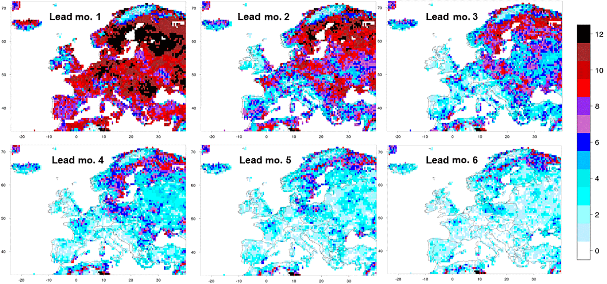
Figure 4Number of months in a year with significant skill (R) in the run-off forecasts of lead months 1–6.
Figure 4 displays a synthesis in the form of six maps with the number of the 12 months of the year with significant skill for lead months from 1 to 6. In accordance with what was also illustrated by Fig. 2, the amount of significant skill degrades with increasing lead time. There is generally more skill throughout the year towards the north and the northeast. Many of the regions with very little or no skill are coastal regions (e.g. northern coast of Spain), especially coastal regions on the western side of land masses (e.g. western coasts of Denmark, southern Norway, Italy, Croatia and the British Isles), and mountain regions (e.g. the Alps, except for their southern fringe, mountains in northern Norway and Sweden and the Tatras on the border of Poland and Slovakia). The British Isles exhibit little skill, except for the eastern coast of Great Britain in late winter and early spring (JFMA). Many of the regions that were listed before as having consistent skill for lead month 2 also appear as foci of skill during the whole year, namely Fennoscandia, northeast Germany and northwest Poland, Romania and Bulgaria, western France and the eastern side of Great Britain. The companion paper shows that for regions with skill during a large part of the year, this skill is due to initial conditions of snow and/or soil moisture.
These pan-European results can be compared to those of Bierkens and Van Beek (2009). They found maxima in predictability of winter discharge in northern Sweden, Finland, the region between Moscow and the Baltic Sea, Romania and Bulgaria, and eastern Spain. For the winter there is crude agreement with the current study about northern Sweden, Romania and Bulgaria, but not about the other regions. For the summer, Bierkens and Van Beek (2009) compute maxima in skill for southern Spain, Sardinia, western Turkey and southwestern Finland, a pattern that broadly agrees with the locations of the summertime maxima in skill we find (most of Fennoscandia and southern part of the Mediterranean region).
Singla et al. (2012) found considerable skill in the Seine basin for low flows from June to September – a bit more eastern from the region where we found skill. Trigo et al. (2004) using a statistical model based on December NAO indices found skill for JFM discharge (and hydropower production) for the Douro, Tejo and Guadiana basins covering most of central and western Iberia. We confirm this skill for March in these regions, but not for January and February, while we find some skill for later months (March until August). Svensson et al. (2015) using a statistical model, based on NAO indices and river flow persistence, found good skill for winter river flows on the eastern side of the British Isles, consistent with our findings, and low but just significant skill along its western coast, which we do not reproduce.
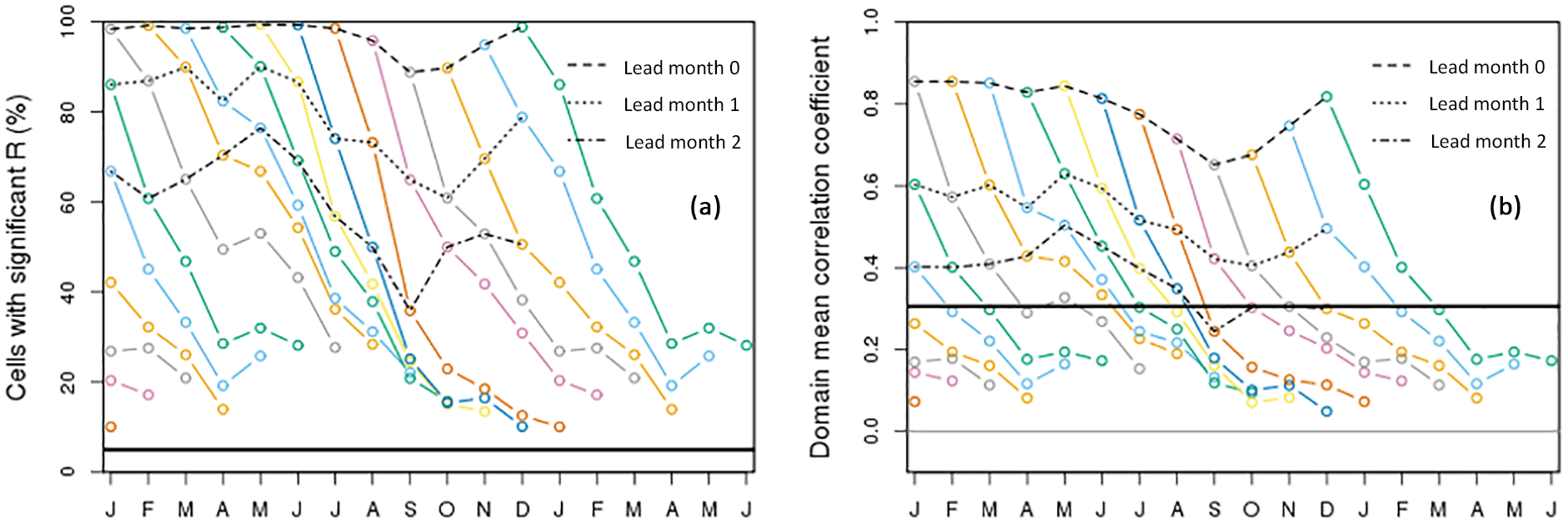
Figure 5(a) Fraction of cells with significant skill (in terms of R), and (b) domain average correlation in the run-off hindcasts, as a function of initialisation month and lead time. Each coloured curve corresponds to the hindcasts initialised in a single month. For better visualisation, parts of the curves that end in the next year are shown twice, namely at the left-hand and the right-hand side of the graph. Black lines (dashed, dotted and dashed–dotted) connect the results for identical lead times. The horizontal line in (a) shows the expected fraction of cells with significant skill, in the case that the hindcasts have no skill at all (5 %), and in (b) the minimal magnitude of the correlation of a single cell for it to be statistically significant.
Figure 5a summarises skill across the domain in terms of the fraction of cells with significant R for all initialisation and lead months. Overall there is a considerable amount of significant skill, with a minimum roughly from August to November and a maximum in May. For lead month 2 the fraction of cells with significant skill varies between 36 % (September) and 76 % (May). In all of the 84 combinations of initialisation and lead month, the theoretical value of no skill at all (5 %) is exceeded, implying that there are (small) pockets of skill even at lead month 6. Individual curves show that skill is lost with increasing lead time. The exception is formed by hindcasts starting in November, December and January which gain skill when they progress from April to May, a phenomenon caused by initial conditions of snow that takes longer or shorter to completely melt in (late) spring. For details, see the companion paper. Figure 5b shows decay and gain trends of the domain-averaged R. It shows that a forecast initialised in February exhibits higher domain average skill into June (5 lead months) than one starting in July into September (2 lead months). Similar summary plots for the other skill metrics are presented in the Fig. S2 and discussed in Sect. 3.4.
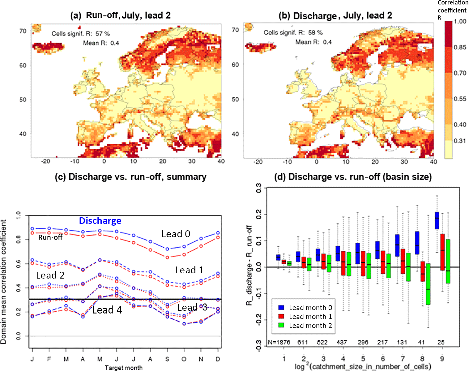
Figure 6Comparison of the performance of the hindcasts of discharge and run-off using the pseudo-observations for verification. The two maps display R for run-off (a) and discharge (b) for hindcasts initialised on 1 May and target month July (see further explanation in Fig. 1). (c) depicts the annual cycle of the domain-averaged R for run-off (red) and discharge (blue) for lead months 0 to 4. The horizontal line at 0.31 is the threshold of significance for a single cell. (d) is a box plot of the difference between R for discharge and run-off as a function of the basin size. Each bin i contains the results for all basins with a maximum of 2i cells and more than 2(i−1) cells; e.g. bin 4 is for all basins with a size from 10 to 16 cells. Boxes represent the interquartile range and the median; whiskers extend to minimum and maximum values found in the bin. All values are average differences over the 12 months of the year and results are shown for three different lead times. The values above the abscissa give the number of cells in each bin.
3.2 Spatio-temporal variation of skill in discharge forecasts
This subsection compares the skill for discharge with the skill for run-off. The two maps of Fig. 6, which depict the skill in run-off and discharge hindcasts for July as lead month 2, show a high degree of similarity in terms of the patterns and the magnitude of the skill. The same holds for other target months and lead times (not shown). There are, however, subtle differences because rivers aggregate the skill, or lack of skill, from the whole upstream part of their basin. As a result, cells containing rivers with large basins may contrast against adjacent cells if these contain rivers with a small, local basin. Indeed, some downstream parts of large rivers stick out in the skill map for discharge, but not in the skill map for run-off. An example in Fig. 6b is the reaches of the Danube along the Romanian–Bulgarian border, which show more skill than local small rivers in adjacent cells, because some upstream parts of the Danube have more skill than the region around the Romanian–Bulgarian border. An example that demonstrates the opposite is the downstream part of the Loire showing less skill than local small rivers, because upstream parts of the Loire have less skill than small, local rivers in the downstream part.
Domain summary statistics of skill also differ slightly between run-off and discharge. Figure 6c compares the annual cycle of the skill in discharge with the skill in run-off at five different lead times. Here we show the difference in the domain-averaged R instead of the fraction of cells with a significant R because in lead month 0 that fraction is close to 1 for both variables. In terms of the domain-averaged R, predictability is higher for discharge than for run-off for the first lead month. On average over the 12 months of the year, the difference is 0.049. We ascribe this result to the combined effect of the delay between run-off and discharge, with variations in discharge being later in time than the corresponding variations in run-off, and the general tendency of decreasing skill with lead time. The curves for the different lead times in Fig. 6c show that the difference in skill between the two variables gradually disappears with increasing lead time (an annual average of 0.020 and 0.012 for lead months 1 and 2, respectively). This is compatible with the given explanation for the difference and the fact that the rate with which skill is lost gradually decreases with increasing lead time.
We finally analysed whether the difference in skill between discharge and run-off was a function of the size of the basin (Fig. 6d). For the first lead month, when on average there is more skill in discharge than in run-off, the difference increases with the size of the basin. Again, this can be explained by the combination of the skill decaying with time and the delay between run-off and discharge, with the delay increasing with the size of the basin. For longer lead times (from lead month 1 on), when the domain-averaged difference in skill has become very small, the figure shows no effect of the basin size. Referring to the comparison between run-off and discharge in panels Fig. 6a and b for lead month 2, cases like the Danube (more skill than local rivers) and the Loire (less skill than local rivers) tend to cancel out when the entire domain and year are considered.
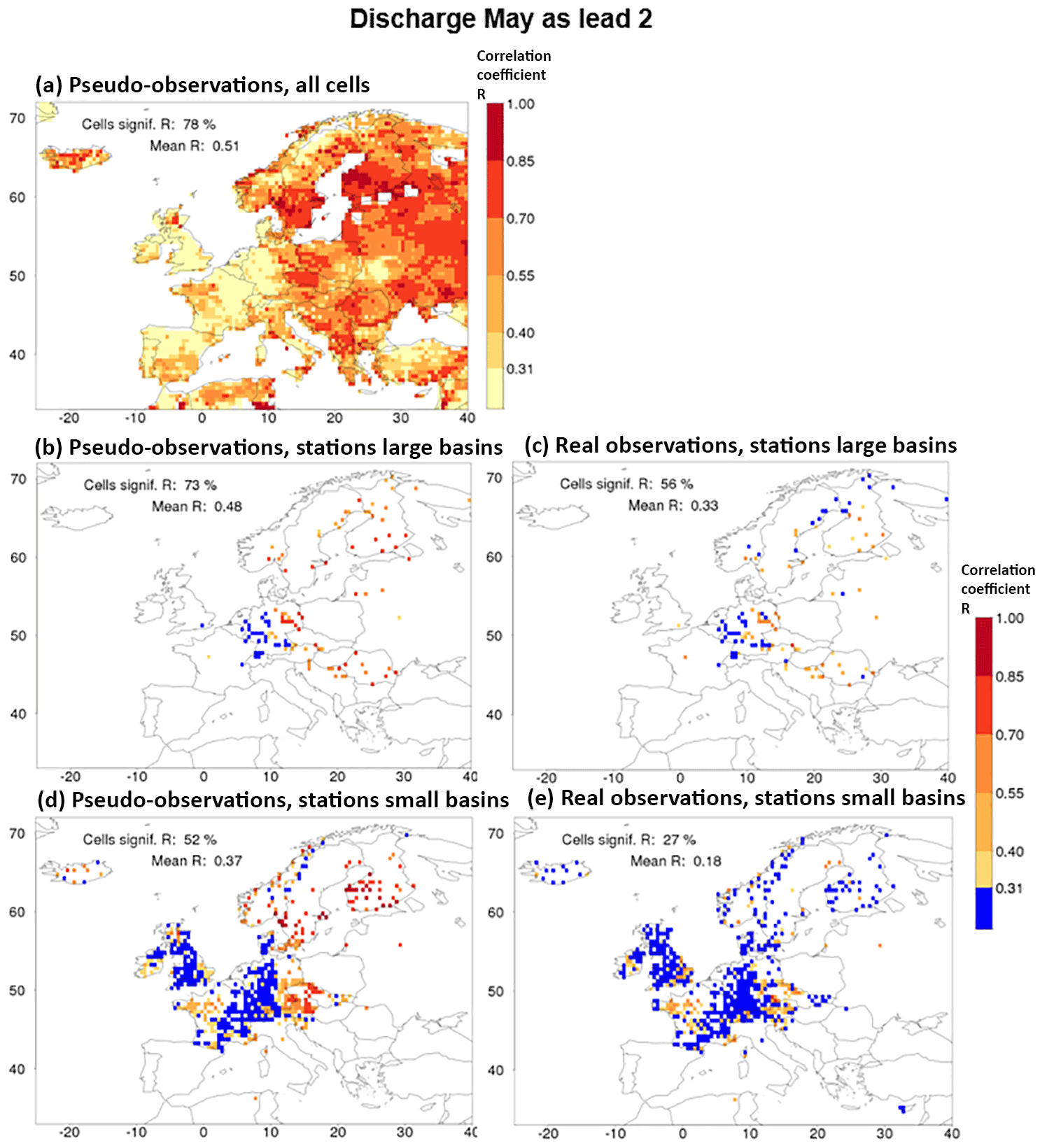
Figure 7Skill (R) of the discharge hindcasts for May as lead month 2 (initialisation on 1 March). In sequence: (a) discharge verified with pseudo-observations; (b) as (a) but for cells with real observations representing large basins only; (c) discharge verified with real observations for large basins. (d) and (e) are identical to (b) and (c), respectively, but for cells with real observations representing small basins. More explanation is given in the caption of Fig. 1, but in (d) and (e) cells with insignificant skill are coloured blue instead of yellow for better contrast.
3.3 Verification of discharge with pseudo- and real observations
So far, all skill was determined by using the discharge generated with the reference simulation. i.e. with pseudo-observations. In this section, this theoretical skill will be compared with the skill determined with real discharge as observed at gauging stations (actual skill) from the GRDC and EWA databases. Figure 7 compares the theoretical skill (Fig. 7b and d for large and small basins, respectively) with actual skill (Fig. 7c and e for large and small basins, respectively) for a single combination of a target month (May) with a lead month (2). Small basins are defined as smaller than one 0.5∘ × 0.5∘ grid cell; large basins are larger than 9900 km2 (see Sect. 2.2).
For this combination of May forecasts initialised in March, a substantial degradation in skill is found when the pseudo-observations are replaced by real observations. In terms of the fraction of cells with significant skill, the reduction is from 73 to 56 % for large basins and from 52 to 27 % for small basins and the domain-averaged R decreases from 0.48 to 0.33 for large basins and from 0.37 to 0.18 for small basins. In particular, the basins in northern Fennoscandia lose much of their skill when using actual instead of pseudo-observations. In this region VIC also performed poorly in reproducing historic flows. Specific discharge was underestimated and the annual cycle was poorly reproduced, especially the spring peak occurred too late and lasted too long (Greuell et al., 2015). In central Europe useful skill remains when using real observations for both small and large basins. This is a region where VIC reproduced annual cycles well, though inter-annual variations in low flows were overestimated. For a few stations in northwest France and southeast England actual skill is larger than theoretical skill.

Figure 8Comparison between verification of discharge with pseudo- (red) and real (blue) observations in terms of the annual cycle of the domain-mean R. The horizontal line at 0.31 is the threshold of significance for a single cell. Results are shown for cells representing large basins (a) and cells representing small basins (b). Both panels depict cycles for lead months 0 and 2 only.
Figure 8 compares actual with theoretical skill for all target months and two lead times by considering the domain-mean R. Similar figures for the other skill metrics are presented in Fig. S4 and discussed in the next section. The reduction of actual relative to theoretical skill occurs for all combinations of target and lead months and does not exhibit a clear annual cycle. On average across all target months and for lead month 2, the ratio of actual to theoretical skill is 0.667 (0.258 divided by 0.387) for large basins and 0.538 (0.156 divided by 0.290) for small basins. This is comparable to Van Dijk et al. (2013), who found a ratio of actual to theoretical skill of 0.54 for 6192 basins worldwide in terms of the ranked correlation coefficient.
Comparing skill for small basins with skill for large basins in Fig. 8, we notice two differences. Firstly, in terms of the domain-mean R, theoretical skill is higher for large basins than for small basins (0.39 and 0.29, respectively, for the annual mean and lead month 2). However, this result holds for the cells with observations. If all cells of the domain are considered, this difference becomes insignificantly small. So, the apparent difference in theoretical skill between large and small basins can be attributed almost entirely to the geographical distribution of the discharge monitoring stations, with stations on small basins being more often located in regions with relatively little skill, such as Germany, France and the British Isles, than large basin stations.
The second effect of the size of basins is that the ratio between theoretical and actual skill is larger for small basins than for large basins, at least for lead month 0. This is perhaps even more clear from Fig. S3 in the Supplement. We speculate that this is due to a combination of two effects. Firstly, there is more skill in simulations of historic streamflow in large basins than in small basins (Van Dijk and Warren, 2010, confirmed for VIC in Europe by Greuell et al., 2015). Secondly, as Van Dijk et al. (2013) demonstrated, the ratio of actual to theoretical skill in the hindcasts is almost linearly related to the skill of simulating historic streamflow. Combining these two relationships confirms the relationship that we found, namely an increase in the ratio of actual to theoretical skill with basin size.
Finally, we investigated to what extent these results are affected by human interference, keeping in mind that the simulations are natural, while the observations include human impacts to a variable but unknown degree. Human interference is expected to have a negative effect on actual skill and hence on the ratio of actual to theoretical skill. For relatively natural large basins (AAPFD < 0.3; see end of Sect. 2.2), the ratio of actual to theoretical skill was computed in terms of the domain-mean R, averaged across all target months and for lead month 2. We found a ratio of 0.686, which should be compared to a ratio of 0.667 for the entire set of large basins (see above). So, as expected the ratio is larger for basins with less impact. However, since the difference between the two ratios is small we conclude that the effect of evaluating natural runs against observations that are obviously affected by human interference contributes only little to the difference between actual and theoretical skill. A similar analysis was not applied to the collection of small basins with observations, since these are smaller than the spatial resolution of the simulations.
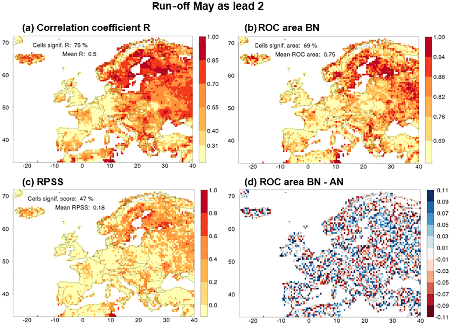
Figure 9Maps of different skill metrics for one combination of a target month (May) and a lead month (2) of the run-off hindcasts. Panels show (a) R, (b) the ROC area for the below-normal tercile, (c) the ranked probability skill score (RPSS) and (d) the difference in ROC area between the BN and AN terciles. (a, b, c) skill is not significant in cells with a yellow colour. Legends provide the fraction of cells with significant values of the metric and the domain-averaged value of the metric.
3.4 Results for other skill metrics
So far, skill was measured in terms of the correlation coefficient between the median of the hindcasts and the observations (R) only. This section compares those results, for run-off, with results in terms of other skill metrics. Figure 9 gives an example for one particular target month and lead month, i.e. target May initialised in March (lead 2). Figure 9a–c show the skill patterns for R, for the ROC area for below-normal (BN) years and for the RPSS. The three patterns are spatially similar to a large degree, though the magnitudes and number of significant cells do differ. The pattern of the map of the ROC area for above-normal (AN) years (see Fig. S1) is also similar to the patterns of the three maps shown. On average across all lead and target months, among cells that have significant R, 89 and 84 % also have a significant ROC score for the BN tercile and the AN tercile, respectively, and 65 % also have significant RPSS scores. The fraction of cells with no significant R, but with significant ROC or RPSS, remains below the 5 % level across all target and lead months.
The agreement that we find between the patterns of the different metrics is in accordance with a result mentioned in a global analysis of seasonal streamflow predictions by Van Dijk et al. (2013), who found high spatial correlation between the different skill metrics they used (among which were R, the RPSS and the ranked correlation coefficient).
Although the different nature of the different metrics makes the interpretation of quantitative differences between them difficult, this is not true for the ROC areas for the different terciles. For the particular combination of May as target month and lead month 2 shown in Fig. 9, the domain-mean ROC area is largest for the BN tercile (0.75), slightly smaller for the AN tercile (0.73) and much lower for the near-normal tercile (0.58, see Fig. S2c and d). A similar tendency is found in the fraction of cells with a significant ROC area (69, 63 and 21 %, respectively). In fact, in all combinations of lead and target month the fraction of significant cells is larger for the BN than for the AN tercile, as shown in Fig. 10. However, the AN and BN fractions of cells tend to become equal (i) when they approach 1.0, (ii) when they approach the limit of no skill (5 %) and (iii) during target months from October to January. Finally, Fig. 9d presents a map of the difference between the BN and the AN ROC area for May as lead month 2. There is some organisation in the pattern but regions with a positive or a negative difference between the two tend to be smaller than the regions with significant skill in the maps of, for example, Figs. 2 and 3. Also, we did not detect much consistency, in the sense of persistence during at least two consecutive target or lead months, in the patterns of the difference between ROC AN and ROC BN.
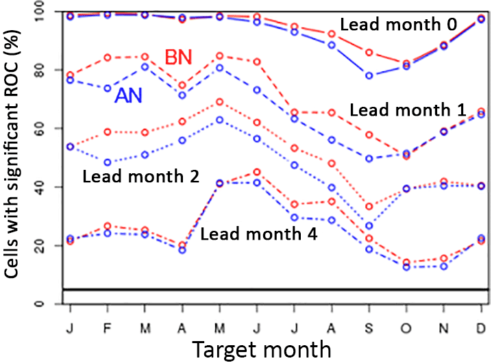
Figure 10Skill of the run-off hindcasts in the below-normal (BN) tercile compared to the skill of the run-off hindcasts in the above-normal (AN) tercile. The plot depicts annual cycles of the fraction of cells with a significant ROC area for the two terciles and for 4 lead months.
In Fig. 9c the fraction of cells with a significant value of the RPSS is 47 %, which is somewhere between the fractions for ROC areas of the three terciles because the RPSS represents the skill across all terciles.
For other combinations of target and lead months the results of this analysis are qualitatively similar (see Supplement figures). All metrics show a minimum value in the annual cycles in either September or in October, irrespective of lead time; maxima are attained in February for lead month 0 shifting to May at longer lead times (Fig. S2). We would finally like to note that, while in this subsection we discussed run-off, we made similar figures and calculations for discharge. Results for these two variables are almost identical.
4.1 Theoretical versus actual skill
In the analysis of the differences between theoretical and actual skill, two essential questions are as follows. (a) What are the conceptual differences between the physical systems that generate the pseudo- and the real discharge observations, i.e. between the model reference run and the real world? To answer this question, the components in the upper and the lower box of the diagram in Fig. 1 need to be compared. (b) What are the expected effects of these differences on skill, i.e. on the comparison with the hindcasts? To answer this question, the components that differ between the real world and the model reference run need to be compared with the model hindcasts. The rule then is that skill decreases with increasing disagreement between a component of the hindcast system and the corresponding component of one of the other systems. The following components differ between the real world and the model reference simulation.
(1) Real meteorology differs from the meteorology assumed in the reference simulation (WFDEI), both during the spin-up period and during the hindcast period. During spin-up, the model reference run and hindcasts have identical meteorological forcing (WFDEI), which differs from real meteorology. Therefore, this difference is expected to lead to more theoretical than actual skill. During the hindcast period, all three systems have different meteorological forcing. We do not have a well-founded expectation about any biases between these three forcings and, hence, we have no expectation about its effect on the difference between theoretical and actual skill. However, in Europe and beyond the first lead month, almost all skill in the seasonal forecasts is due to the initial conditions (see the companion paper). Therefore, beyond the first lead month and in Europe, differences in forcing during the hindcast period have a negligible effect on skill.
(2) Models are imperfect, in terms of physics and in terms of spatial and temporal discretisation, so model hydrology differs from real world hydrology. Hindcasts and the pseudo-observations are produced with the same model, so imperfections in model hydrology are expected to lead to more theoretical than actual skill. One assumption implicitly made in the diagram is that the basin of the observation station and the model basin are identical. This is not the case (see Sect. 2.2), so differences between observation and model basin form an additional cause of disagreements between theoretical and actual skill. Again, this will favour theoretical skill with respect to actual skill since basins are identical in the hindcasts and the reference simulation. In particular, differences in meteorological forcing between the basin of the observation station and the model basin might reduce actual skill. Van Dijk et al. (2013) investigated this aspect by making simulations for Australia at different spatial resolutions and verifying with networks of observations with different spatial densities. They found that the resolution and perhaps the quality of the forcing data contributed at least half to the difference between theoretical and actual skill.
(3) In the real world discharge observations are subject to measurement errors. Measurement errors of discharge are not constant over time (due to varying cross sectional areas, following erosion and sedimentation) and therefore add noise to the data; noise always reduces skill. There is no equivalent of this error in the model environment. Hence, as for differences (1) and (2) this difference is expected to lead to more theoretical than to actual skill.
(4) Initial conditions are absent in this list of differences since they are not independent components but entirely determined by two components of the system listed above, namely meteorology and hydrology. Alternatively, initial hydrological conditions could be taken from observations or by assimilation of observations into model calculations. In that case, initial conditions would become an independent or semi-dependent component of the system. However, while model initial conditions would, of course, differ from real initial conditions, the two model systems had identical initial conditions. Hence, this difference would again be expected to lead to more theoretical than to actual skill.
In summary, all of the conceptual differences between the generation of pseudo- and real observations are expected to lead to more theoretical skill than actual skill, except for the difference in meteorology during the hindcast period, which has, in the case of Europe beyond the first lead month, a neutral effect, and otherwise an unknown effect.
Our data analysis, Sect. 3.3, broadly confirms that theoretical skill exceeds actual skill. We also found cases where actual skill exceeds theoretical skill beyond lead month 0, such as for a few stations in northwest France and southeast England in Fig. 7. We ascribe such cases to chance.
It is interesting to discuss what would happen in the utopian case that the system of the model reference run would converge with the real world, i.e. if model meteorological forcing and hydrology would approach perfection and if measurement errors would approach zero. Equality of the two systems would, according to the analysis above, lead to equality of theoretical and actual skill. However, we like to note that at the same time optimisation of the model system can lead to a degradation of the theoretical skill due to unrealistic memory timescales in the storage compartments of the hydrological model before optimisation. If this memory, from stored water in either snow, soil or aquifer, is too strong, then skill would decrease with the calibration of the model towards more realistic storage accumulation. However, if this memory is too small before improving the model, then, of course, the reverse would happen and skill would increase with optimisation.
An example proving this statement is a model that accumulates too much snow. The model will do so both in the initial state of the reference simulation and the initial state of the hindcasts, and, since more snow leads, at some stage of the melting season, to more predictive skill, theoretical skill will be overestimated. A perfect model, accumulating less but more realistic amounts of snow, would exhibit less skill. Another example is predictive skill caused by inter-annual variations in the initial amount of soil moisture and/or groundwater. A model that is imperfect because it overestimates the transport speed of water through the soil and the groundwater reservoirs will do so both in the reference simulation and the hindcasts. Predictive skill due to soil moisture initial conditions will then occur too early. Compared to the model that overestimates transport speed, a perfect model with smaller, realistic transport speed would yield less theoretical skill at the early lead times.
Hence, theoretical skill is not equal to the maximum that could be accomplished if hydrological model and meteorological forcing during the reference simulation were perfect.
The version of VIC used in this study was calibrated by Nijssen et al. (2001) in a crude way, in the sense that they assumed no spatial variation of the parameters set by calibration within almost the entire European continent. Improving the calibration of VIC would be an obvious candidate for trying to improve the seasonal predictions discussed in this paper. This should lead to higher actual skill. However, the two examples discussed above show that theoretical skill may actually, for certain locations, months of initialisation and lead months, decline due to the recalibration.
4.2 Results and uncertainties
There seems to be a broad correspondence between the probabilistic forecast verification presented here and the model validation presented in Greuell et al. (2015) and Roudier et al. (2016). These studies found that average discharge and inter-annual variations therein are well reproduced against observations, consistent with our result that in the first lead month all skill scores, also against real observations (see Fig. S4 for the lead 0 results), are good for large parts of Europe.
However, the relation between a model's ability to simulate historic streamflow and its ability to generate skill in seasonal forecasts is complex. There is, for instance, no reason to expect that regions with more theoretical skill than other regions would generally correspond to regions with better historic streamflow simulations. Large model stores of soil moisture and snow tend to lead to more theoretical skill, whether these stores are realistic or not. If they are not realistic, simulations of historic streamflow will be poor, despite the forecast skill. Another example of the problematic relation between validation and verification is that, even in perfect models, regions with small model stores of soil moisture and snow and regions with large inter-annual variation in precipitation will exhibit small amounts of theoretical and actual skill. So, regions with high-quality historic streamflow simulations may for good reasons have little skill in the forecasts.
However, what we would expect is that regions of poor model performance have little actual skill (not necessarily little theoretical skill) in the forecasts. In our work, this statement is broadly confirmed by the basins in northern Fennoscandia, which lose much of their skill when using actual instead of pseudo-observations (Fig. 7). In this region VIC indeed performed poorly in reproducing historic flows. Good model performance probably is a necessary (but not sufficient) condition for the generation of actual skill in seasonal forecasts. This is exemplified by some regions with considerable amounts of actual skill in central Europe (e.g. northern part of the Balkans and the Elbe basin in Fig. 7), where VIC's simulations of historic streamflow are much better than in northern Fennoscandia.
In a future extension of our work, an objective method like cluster analysis could reveal regions where skill has a similar signature. This could lead to an improved assessment of the physical and climatological factors that are responsible for the spatial variations in skill found in this and its companion paper.
There also seems to be a broad correspondence between the regions and seasons with skill identified in the present work and those identified in more spatially or temporally confined studies based on entirely different physical or even statistical models. Without repeating the more detailed description in the introduction and the closer comparison in Sect. 3.1, we restate here that the results of Bierkens and van Beek (2009) and Thober et al. (2015) were similar at the European domain. These pan-European studies, like ours, confirm more regional studies such as those for the British Isles (Svensson et al., 2015) or France (Céron et al., 2010; Singla et al., 2012). Though a high-resolution study like the latter may add much spatial detail, this does not change the region and season of skill.
Our results are based on a forcing with the 15-member, monthly initialised, 7-month forecast version of ECMWF System 4, basically because at the start of this work that hindcast was the only one accessible to us, but also because it allows verification at the monthly resolution. Alternatively, we could have used the 51-member seasonally initialised (4 times per year), 7-month forecast version of the same model. That would have provided us with better-constrained, more-precise statistics (larger sample size), or it would have allowed assessment of more percentiles (e.g. quintiles instead of terciles) at similar precision. However, the variation of skill over a year would not have been resolved with such detail as in the present work. Finally, a 15-member, seasonally initialised, 12-month forecast version of System 4 is available. Our results show that for some regions at lead month 6, still a few, small pockets of consistent skill remain, suggesting that extending the forecast for our domain might be worth exploring.
Other seasonal forecasting systems, based on different coupled ocean–climate models, could have been used as meteorological forcing, such as CFSv2 (Saha et al., 2014) and GloSea5 (MacLachlan et al., 2014). Given that, at least at large scales, multi-model ensembles exhibit better climate forecast skill than single models, it is interesting to investigate whether that additional skill also propagates into river flow forecasts. While this seems to be true for the eastern United States (Luo and Wood, 2008), it is not known whether similar conclusions could be drawn for Europe. A similar reasoning can also be extended to the hydrological models: using a multi-climate model ensemble to force a multi-hydrological model ensemble might also provide improved skill, as the latter models may be complementary in the regions and seasons of best model performance. Bohn et al. (2010) showed some advantage of using an ensemble of three hydrological models (but with a single forcing), over using only the best of the three, but only after bias correcting the hydrological output and making a linear combination of them with monthly varying weights.
4.3 Implications and recommendations
Many conclusions drawn from this work are valid at the scale of our domain and not necessarily at the scale of river basins. Only in some parts of our analysis, especially where we focused on the annual cycle of the skill (Fig. 3), regional patterns at a scale smaller than that of the domain were discussed. This was done in a qualitative way.
For applications of these seasonal forecasts in decision-making processes at (sub-)basin level, a more detailed skill analysis is recommended for that specific (sub-)basin, preferably after a better model calibration for that same basin. The facts presented in this study that anomaly correlations and ROC scores for the AN and BN terciles are significant for large parts of the domain for lead times up to several months, supported by (fairly) positive validation results for VIC (Greuell et al., 2015; Roudier et al., 2016), suggest these anomaly forecasts are good enough to be used as such. However, areas of significant RPSS are much smaller and remain significant for shorter lead times. Spatially distributed calibration of VIC model parameters, or distribution-based calibration of modelled discharge to observations, or both, might also increase the RPSS. This might then allow forecasting of absolute discharge magnitudes and thus inform decision-making processes that involve certain absolute discharge thresholds.
In Sect. 3 (results) we already discussed the probable reasons for skill, which are much elaborated on in the companion paper. In general, that paper shows that for most areas, skill in run-off is caused by initialising snow and/or soil moisture properly; only in few areas and seasons does skill in precipitation or skill in temperature and evapotranspiration add skill to run-off forecasts beyond the first lead month. This has two implications: one is that, if ever the skill of seasonal climate forecasts improves for Europe, this may well translate to improved seasonal river flow forecast too. The second is that better initial conditions of snow water equivalent and soil moisture from observations may do the same, with the latter happening only if the spatial distribution of the soil moisture storage capacity is more realistic too (see Sect. 4.1).
Overall the present analysis shows that, especially in winter, spring and early summer, there is potentially good skill to forecast run-off and discharge in large parts of Europe, with considerable lead time. While this broadly confirms previously published work, the present study (while being specific to our model set-up) gives much more spatial and temporal (season and lead time) details. As such it provides a good basis to support operational forecasts and to add information about skill to seasonal forecasts, which is very important for proper value assessment and decision making.
This paper is the first of two papers dealing with a model-based system built to produce seasonal hydrological forecasts (WUSHP: Wageningen University Seamless Hydrological Predictions). The present paper presents the development and the skill evaluation of the system for Europe; the companion paper provides an explanation of the skill or the lack thereof.
First, theoretical skill of the run-off hindcasts was determined using the output of the reference simulation as pseudo-observations. Using the correlation coefficient (R) as metric, hot spots of significant skill were found in Fennoscandia (from January to October), the southern part of the Mediterranean (from June to August), Poland, northern Germany, Romania and Bulgaria (mainly from November to January), and western France (from December to May). There is very little or no significant skill throughout the year in some coastal and mountainous regions. The entire British Isles exhibit very little skill, except for the eastern coast of Great Britain. If the entire domain is considered, the annual cycle of skill has a minimum roughly from August to November and a maximum in May.
Run-off and discharge show a high degree of similarity in terms of the spatial patterns and the magnitude of the skill. However, when averaged over the domain and the year, predictability is slightly higher for discharge than for run-off for the first lead month (by 0.049 in terms of R), but the difference decreases with increasing lead time. We also found that for lead month 0 the difference between discharge and run-off skill increases with the size of the basin.
Theoretical skill as determined with the pseudo-observations was compared to actual skill as determined with real discharge observations. On average across all target months and for lead month 2, skill reduction due to replacing pseudo- by real observations is larger for small basins than for large basins.
Spatio-temporal patterns for the different skill metrics considered in this study (correlation coefficient, ROC area and ranked probability skill score) are similar to a large degree. ROC areas tend to be slightly larger for the below-normal tercile than for the above-normal tercile but not during target months from October to January.
The data from WUSHP are available to researchers upon request. Please visit https://www.wur.nl/en/Research-Results/Chair-groups/Environmental-Sciences/Water-Systems-and-Global-Change-Group.htm for more details.
The supplement related to this article is available online at: https://doi.org/10.5194/hess-22-3453-2018-supplement.
WG and RWAH designed the experiments, with suggestions from the other co-authors. WHPF and WG developed the workflow scripts and performed all the simulations. WG and WHPF developed the analyses and plotting scripts in R. HB did the LPJmL work on AAPFD. All co-authors participated in repeated discussions on interpretations of results and suggested ways forward in the analysis. WG prepared the first version of the manuscript with contributions from all co-authors. RWAH and WG prepared revisions of the manuscript with contributions from all co-authors.
The authors declare that they have no conflict of interest.
This article is part of the special issue “Sub-seasonal to seasonal hydrological forecasting”. It is not associated with a conference.
This study was financially supported by the EUPORIAS project (EUropean
Provision of Regional Impact Assessment on Seasonal-to-decadal timescale) –
grant agreement no. 308291, funded by the European Commission (EU) project
in the Seventh Framework Programme. We thank the valued suggestions and
insightful comments from two (anonymous) reviewers that contributed to an
improved version of the manuscript.
Edited by: Ilias Pechlivanidis
Reviewed by: Christel Prudhomme and two anonymous referees
Alfieri, L., Pappenberger, F., Wetterhall, F., Haiden, T., Richardson, D., and Salamon, P.: Evaluation of ensemble streamflow predictions in Europe, J. Hydrol., 517, 913–922, 2014.
Bhend, J., Ripoldi, J., Mignani, C., Mahlstein, I., Hiller, R., Spirig, C., Liniger, M., Weigel, A., Bedia Jimenez, J., De Felice, M., Siegert, S., and easyVerification: Ensemble Forecast Verification for Large Data Sets, available at: https://CRAN.R-project.org/package=easyVerification, 2016.
Bierkens, M. F. P. and Van Beek, L. P. H.: Seasonal predictability of European discharge: NAO and hydrological response time, J. Hydrometeorol., 10, 953–968, 2009.
Bohn, T. J., Sonessa, M. Y., and Lettenmaier, D. P.: Seasonal Hydrologic Forecasting: Do Multimodel Ensemble Averages Always Yield Improvements in Forecast Skill?, J. Hydrometeorol., 11, 1358–1372, 2010.
Bruno Soares, M. and Dessai, S.: Barriers and enablers to the use of seasonal climate forecasts amongst organisations in Europe, Clim. Change 137, 89–103, 2016.
Céron, J. P., Tanguy, G., Franchistéguy, L., Martin, E., Regimbeau, F., and Vidal, J.-P.: Hydrological seasonal forecast over France: feasibility and prospects, Atmos. Sci. Lett., 11, 78–82, 2010.
Crochemore, L., Ramos, M.-H., and Pappenberger, F.: Bias correcting precipitation forecasts to improve the skill of seasonal streamflow forecasts, Hydrol. Earth Syst. Sci., 20, 3601–3618, https://doi.org/10.5194/hess-20-3601-2016, 2016.
Demirel, M. C., Booij, M. J., and Hoekstra, A. Y.: The skill of seasonal ensemble low-flow forecasts in the Moselle River for three different hydrological models, Hydrol. Earth Syst. Sci., 19, 275–291, https://doi.org/10.5194/hess-19-275-2015, 2015.
Doblas-Reyes, F. J., García-Serrano, J., Lienert, F., Biescas, A. P., and Rodrigues, L. R.: Seasonal climate predictability and forecasting: status and prospects, Wiley Interdisciplinary Reviews, Clim. Change, 4, 245–268, 2013.
Döll, P. and Lehner, B.: Validation of a new global 30-min drainage direction map, J. Hydrol., 258, 214–231, 2002.
ECMWF Seasonal Forecast User Guide, retrieved from: http://www.ecmwf.int/en/forecasts/documentation-and-support/long-range/seasonal-forecast-documentation/user-guide/introduction, last access: October 2016.
Ghile, Y. B. and Schulze, R. E.: Development of a framework for an integrated time-varying agrohydrological forecast system for Southern Africa: Initial results for seasonal forecasts, Water SA, 34, 315–322, 2008.
Greuell, W., Andersson, J. C. M., Donnelly, C., Feyen, L., Gerten, D., Ludwig, F., Pisacane, G., Roudier, P., and Schaphoff, S.: Evaluation of five hydrological models across Europe and their suitability for making projections under climate change, Hydrol. Earth Syst. Sci. Discuss., 12, 10289–10330, https://doi.org/10.5194/hessd-12-10289-2015, 2015.
Greuell, W., Franssen, W. H. P., and Hutjes, R. W. A.: Seasonal streamflow forecasts for Europe – II. Explanation of the skill, Hydrol. Earth Syst. Sci. Discuss., https://doi.org/10.5194/hess-2016-604, in review, 2016.
Hagedorn, R., Doblas-Reyes, F. J., and Palmer, T. N.: The rationale behind the success of multi-model ensembles in seasonal forecasting – I. Basic concept, Tellus A, 57, 219–233, 2005.
Hamlet, A. F., Huppert, D., and Lettenmaier, D. P.: Economic value of long-lead streamflow forecasts for Columbia River hydropower, J. Water Res. Plan. Manage., 128, 91–101, 2002.
Haylock, M. R., Hofstra, N., Klein Tank, A. M. G., Klok, E. J., Jones, P. D., and New, M.: A European daily high-resolution gridded data set of surface temperature and precipitation for 1950–2006, J. Geophys. Res.-Atmos., 113, 1984–2012, 2008.
Juston, J., Jansson, P. E., and Gustafsson, D.: Rating curve uncertainty and change detection in discharge time series: case study with 44-year historic data from the Nyangores River, Kenya, Hydrol. Proc., 28, 2509–2523, 2014.
Koster, R. D., Mahanama, S. P., Livneh, B., Lettenmaier, D. P., and Reichle, R. H.: Skill in streamflow forecasts derived from large-scale estimates of soil moisture and snow, Nat. Geosci., 3, 613–616, 2010.
Lehner, B., Reidy Liermann, C., Revenga, C., Vörösmarty, C., Fekete, B., Crouzet, P., Döll, P., Endejan, M., Frenken, K., Magome, J., Nilsson, C., Robertson, J., Rödel, R., Sindorf, N., and Wisser, D.: High resolution mapping of the world's reservoirs and dams for sustainable river flow management, Front. Ecol. Environ., 9, 494–502, 2011.
Li, H.,, Luo, L., and Wood, E. F.: Seasonal hydrologic predictions of low-flow conditions over eastern USA during the 2007 drought, Atmos. Sci. Lett., 9, 61–66, 2008.
Liang, X., Lettenmaier, D. P., Wood, E. F., and Burges, S. J.: A simple hydrologically based model of land surface water and energy fluxes for general circulation models, J. Geophys. Res.-Atmos., 99, 14415–14428, 1994.
Luo, L. and Wood, E. F.: Use of Bayesian Merging Techniques in a Multimodel Seasonal Hydrologic Ensemble Prediction System for the Eastern United States, J. Hydrometeor., 9, 866–884, doi:10.1175/2008JHM980.1, 2008.
MacLachlan, C., Arribas, A., Peterson, K. A., Maidens, A., Fereday, D., Scaife, A. A., Gordon, M., Vellinga, M., Williams, A., Comer, R. E., Camp, J., Xavier, P., and Madec, G.: Global Seasonal forecast system version 5 (GloSea5): a high-resolution seasonal forecast system, Q. J. Roy. Meteor. Soc., 1072–1084, doi:10.1002/qj.2396, 2014.
Marchant, R. and Hehir, G.: The use of AUSRIVAS predictive models to assess the response of lotic macroinvertebrates to dams in south-east Australia, Freshwater Biol., 47, 1033–1050, 2002.
Mason, S. J. and Stephenson, D. B.: How do we know whether seasonal climate forecasts are any good?, in: Seasonal Climate: Forecasting and Managing Risk, Springer Netherlands, 259–289, 2008.
Mo, K. C. and Lettenmaier, D. P.: Hydrologic prediction over the conterminous United States using the national multi-model ensemble, J. Hydrometeorol., 15, 1457–1472, 2014.
Molteni, F, Stockdale, T., Balmaseda, M., Balsamo, G., Buizza, R., Ferranti, L., Magnusson, L., Mogensen, K., Palmer, T., and Vitart, F.: The new ECMWF seasonal forecast system (System 4), ECMWF Technical Memorandum, 656, 2011.
Mushtaq, S., Chen, C., Hafeez, M., Maroulis, J., and Gabriel, H.: The economic value of improved agrometeorological information to irrigators amid climate variability, Int. J. Climatol., 32, 567–581, 2012.
Nijssen, B., O'Donnell, G. M., Lettenmaier, D. P., Lohmann, D., and Wood, E. F.: Predicting the discharge of global rivers, J. Climate, 14, 3307–3323, 2001.
Rost, S., Gerten, D., Bondeau, A., Lucht, W., Rohwer, J., and Schaphoff, S.: Agricultural green and blue water consumption and its influence on the global water system, Water Resour. Res., 44, doi:10.1029/2007WR006331, 2008.
Roudier, P., Andersson, J. C. M., Donnellly, C., Feyen, L., Greuell, W., and Ludwig, F.: Projections of future floods and hydrological droughts in Europe under a + 2∘C global warming, Clim. Change, 135, 341–355, 2016.
Saha, Suranjana and Coauthors: The NCEP Climate Forecast System Version 2, J. Climate, 27, 2185–2208, doi:10.1175/JCLI-D-12-00823.1, 2014.
Schaphoff, S., Heyder, U., Ostberg, S., Gerten, D., Heinke, J., and Lucht, W.: Contribution of permafrost soils to the global carbon budget, Environ. Res. Lett., 8, 014026, doi:10.1088/1748-9326/8/1/014026, 2013.
Sheffield, J., Wood, E. F., Chaney, N., Guan, K., Sadri, S., Yuan, X., and Ogallo, L. A.: drought monitoring and forecasting system for sub-Sahara African water resources and food security, Bull. Am. Meteor. Soc., 95, 861–882, 2014.
Shukla, S. and Lettenmaier, D. P.: Seasonal hydrologic prediction in the United States: understanding the role of initial hydrologic conditions and seasonal climate forecast skill, Hydrol. Earth Syst. Sci., 15, 3529–3538, https://doi.org/10.5194/hess-15-3529-2011, 2011.
Shukla, S., McNally, A., Husak, G., and Funk, C.: A seasonal agricultural drought forecast system for food-insecure regions of East Africa, Hydrol. Earth Syst. Sci., 18, 3907–3921, https://doi.org/10.5194/hess-18-3907-2014, 2014.
Siegert, S., Bhend, J., Kroener, I., and De Felice, M.: SpecsVerification: Forecast Verification Routines for Ensemble Forecasts of Weather and Climate, available at: https://CRAN.R-project.org/package=SpecsVerification (last access: August 2015), 2014.
Singla, S., Céron, J.-P., Martin, E., Regimbeau, F., Déqué, M., Habets, F., and Vidal, J.-P.: Predictability of soil moisture and river flows over France for the spring season, Hydrol. Earth Syst. Sci., 16, 201–216, https://doi.org/10.5194/hess-16-201-2012, 2012.
Svensson, C., Brookshaw, A., Scaife, A. A., Bell, V. A., Mackay, J. D., Jackson, C. R., Hannaford, J., Davies, H. N., Arribas A., and Stanley, S.: Long-range forecasts of UK winter hydrology, Environ. Res. Lett., 10 064006, https://doi.org/10.1088/1748-9326/10/6/064006, 2015.
Themeßl, M. J., Gobiet, A., and Leuprecht, A.: Empirical-statistical downscaling and error correction of daily precipitation from regional climate models, Int. J. Climatol., 31, 1530–1544, 2011.
Thober, S., Kumar, R., Sheffield, J., Mai, J., Schäfer, D., and Samaniegoet, L.: Seasonal Soil Moisture Drought Prediction over Europe Using the North American Multi-Model Ensemble (NMME), J. Hydrometeorol., 16, 2329–2344, 2015.
Trigo, R. M., Pozo-Vázquez, D., Osborn, T. J., Castro-Díez, Y., Gámiz-Fortis, S., and Esteban-Parra, M. J.: North Atlantic oscillation influence on precipitation, river flow and water resources in the Iberian Peninsula, Int. J. Climatol., 24, 925–944, 2004.
Van Dijk, A. I., Peña-Arancibia, J. L., Wood, E. F., Sheffield, J., and Beck, H. E.: Global analysis of seasonal streamflow predictability using an ensemble prediction system and observations from 6192 small basins worldwide, Water Resour. Res., 49, 2729–2746, 2013.
Van Dijk, A. I. J. M. and Warren, G. A.: AWRA Technical Report 4, Evaluation Against Observations, WIRADA/CSIROWater for a Healthy Country Flagship, Canberra, 2010.
Weedon, G. P., Balsamo, G., Bellouin, N., Gomes, S., Best, M. J., and Viterbo, P.: The WFDEI meteorological forcing data set: WATCH Forcing Data methodology applied to ERA-Interim reanalysis data, Water Resour. Res., 50, 7505–7514, 2014.
Wood, A. W. and Lettenmaier, D. P.: A test bed for new seasonal hydrologic forecasting approaches in the western United States, Bull. Am. Meteorol. Soc., 87, 1699–1712, 2006.
Wood, A. W., Hopson, T., Newman, A., Brekke, L., Arnold, J., and Clark, M.: Quantifying Streamflow Forecast Skill Elasticity to Initial Condition and Climate Prediction Skill, J. Hydrometeorol., 17, 651–668, 2016.
Yuan, X., Wood, E. F., Luo, L., and Pan, M.: CFSv2-based seasonal hydroclimatic forecasts over the conterminous United States, J. Climate, 26, 4828–4847, 2013.
Yuan, X., Wood, E. F., and Ma, Z.: A review on climate-model-based seasonal hydrologic forecasting: physical understanding and system development, Wiley Interdisciplinary Reviews: Water, 2, 523–536, 2015.