


Abstract
Most birds engage in extrapair copulations despite great differences across and within species. Besides cost and benefit considerations of the two sex environmental factors have been found to alter mating strategies within or between populations and/or over time. For socially monogamous species, the main advantage that females might gain from mating with multiple males is probably increasing their offspring’s genetic fitness. Since male (genetic) quality is mostly not directly measurable for female birds, (extrapair) mate choice is based on male secondary traits. In passerines male song is such a sexual ornament indicating male phenotypic and/or genetic quality and song repertoires seem to affect female mate choice in a number of species. Yet their role in extrapair mating behavior is not well understood. In this study, we investigated the proportion of extrapair paternity (EPP) in a population of common nightingales Luscinia megarhynchos. We found that EPP rate was rather high (21.5% of all offspring tested) for a species without sexual dimorphism and high levels of paternal care. Furthermore, the occurrence of EPP was strongly related to the spatial distribution of male territories with males settling in densely occupied areas having higher proportions of extrapair young within their own brood. Also, song repertoire size affected EPP: here larger repertoires of social mates were negatively related to the probability of being cuckolded. When directly comparing repertoires sizes of social and extrapair mates, extrapair mates tended to have larger repertoires. We finally discuss our results as a hint for a flexible mating strategy in nightingales where several factors—including ecological as well as male song features—need to be considered when studying reproductive behavior in monogamous species with complex song.
For most passerine species (in 86% of species surveyed), DNA fingerprinting has revealed proportions of extrapair young (EPY) (reviewed in Griffith et al. 2002). This has been also shown for socially monogamous species, although rates of extrapair paternity (EPP) vary strongly among and even within species (reviewed in Petrie and Kempenaers 1998). Several theories have been brought up to explain mating strategies, differing for example in the two sex perspectives. From the male perspective, the main advantage seems obvious since copulations with multiple females usually increase male reproductive success (reviewed in Westneat et al. 1990). Females on the other hand may engage in extrapair copulations (EPC) for genetic benefits for more viable or sexually attractive offspring (reviewed in Andersson 1994; Jennions and Petrie 2000; Schmoll 2011; Wan et al. 2013; but see Akçay and Roughgarden 2007). However, neutral or negative effects of extrapair mating behavior need to be considered, too. For males, seeking EPCs might come at the cost of decreased mate guarding resulting in EPY in their own brood (e.g., Chuang-Dobbs et al. 2001; Akçay et al. 2011). In other species though, males that are successful in siring extrapair offspring are also successful in having more within-pair young (WPY) (e.g., Ferree and Dickinson 2014). For females, EPCs may lead to reduced paternal care or even desertion by the social mate (e.g., Dixon et al. 1994; García-Navas et al. 2013) although in socially monogamous species these effects seem to be less pronounced (reviewed in Møller 2000; Hasselquist and Sherman 2001). Finally, EPCs might also be the result of a mixed mating strategy rather than a specialized reproductive behavior: after having formed a social pair bond, both sexes might additionally engage in extrapair mating whenever the opportunity arises or conditions favor EPCs (e.g., Møller 1985; Magrath and Elgar 1997; Weatherhead 1999).
Here, environmental conditions or ecological factors such as breeding density (reviewed in Westneat et al. 1990; Møller and Birkhead 1993), breeding synchrony (Stutchbury and Morton 1995), weather conditions (Bouwman and Komdeur 2006), food availability (Hoi-Leitner et al. 1999), or habitat structure (Mays and Ritchison 2004; Ramos et al. 2014) can profoundly affect the costs and benefits of extrapair mating behavior, and therefore account for differences across and within species. In particular, the density hypothesis states that EPP should be positively correlated with increased spatial proximity (and therefore increased encounter rates) of individuals (reviewed in Westneat et al. 1990). Although evidence for an effect in interspecific comparison is less consistent, breeding density seems to affect EPP primarily within species (reviewed in Westneat and Sherman 1997). This effect has been found between different populations (Bjørnstad and Lifjeld 1997; Yezerinac et al. 1999) or even between subpopulations (Charmantier and Perret 2004; Stewart et al. 2010; Mayer and Pasinelli 2013). Some investigations found a positive correlation between nearest neighbor distance and EPP (e.g., Møller 1991; Hoi and Hoi-Leitner 1997; Richardson and Burke 1999; Charmantier and Perret 2004) or identified close neighbors as genetic fathers of EYP (e.g., Hasselquist et al. 1996; Kempenaers et al. 1997; Langefors et al. 1998; Foerster et al. 2003).
Another difficulty in the interpretation of results obtained from paternity studies arises from the problem that without detailed behavioral observations it is often not possible to disentangle if EPP is the result of male coercion, or if females actively seek EPCs. Assuming that females actively seek EPCs, it would be expected that they seek higher quality males to do so. Females may assess male quality by pre-copulatory cues such as male secondary sexual traits (reviewed in Jennions and Petrie 2000). Such traits have indeed been found to be linked to male extrapair reproductive success in several species (e.g., Houtman 1992; Møller and Birkhead 1994; Yezerinac and Weatherhead 1997). In passerines, male song is such a sexually selected trait that functions as a condition-dependent indicator of male phenotypic and/or genotypic quality (reviewed in Gil and Gahr 2002). One song parameter that has been intensively studied in this regard is song repertoire size (i.e., the number of distinct elements, syllables, or song types constituting a male’s song). Several studies have shown that large repertoires are related to male quality traits (e.g., Lampe and Espmark 1994; Galeotti et al. 2001; Nowicki et al. 2002; Pfaff et al. 2007). In some species females prefer larger repertoires in song playbacks (e.g., Catchpole et al. 1984; Searcy 1984; Lampe and Saetre 1995) or prefer to mate with large repertoire males (Eens et al. 1991; Reid et al. 2004). However, evidence that repertoire size is also related to EPP is so far very sparse (e.g., reviewed in Garamszegi and Møller 2004).
The nightingale Luscinia megarhynchos is a socially monogamous songbird (Grüll 1981; Glutz von Blotzheim 1989) that has become an established model to study relations between song and male quality (e.g., Kiefer et al. 2006; Kipper et al. 2006; Kunc et al. 2006; Schmidt et al. 2008; Weiss et al. 2012; Sprau et al. 2013; Bartsch et al. 2015a, 2015b). Preliminary findings obtained from a population in the Petite Camarque Alsacienne, France suggest that EPP does occur, but at rather low levels (7.5%; unpublished data PhD thesis Amrhein 2004; see also unpublished data PhD thesis Kunc 2004). So far, we do not know which factors influence extrapair mating behavior in nightingales and whether also song is important in extrapair mate choice. Compared with most other temperate species, nightingale males have extremely large song type repertoires (e.g., Kipper et al. 2004). Yet there is only little knowledge about the role of repertoires during female choice (Kipper et al. 2006). Beyond size, repertoire composition seems to be of importance in nightingale mating contexts. Here, songs containing a peculiar buzz element have been found to show high inter-individual performance differences among males suggesting that singing these songs might be demanding (i.e., high-performance buzzes being difficult to produce). It has indeed been shown that buzz performance is related to male quality (i.e., body measures) in nightingales and a playback experiment revealed that songs containing buzz elements are of particular interest for females (Weiss et al. 2012).
In this study, we analyzed extrapair mating patterns in a nightingale population in Brandenburg (Germany). Having collected data from males including settlement patterns, pairing dates, male age, and song and having analyzed blood samples from all adult territorial males in our study population allows us to address the following topics and questions: firstly, we aimed to characterize the mating behavior in nightingales and expected that EPP would occur in rather low rates as expected from theory and as previously described in another population. Secondly, in a global analysis we aimed to identify parameters, including ecological features as well as male characteristics, which affect extrapairing behavior in our study population. Here, we expected that the distribution of male territories would influence extrapair mating patterns in the way that EPP would occur more often among males that have established territories in close proximity to each other.
Also, we expected that earlier paired and older males should suffer less from cuckoldry assuming that these males represent the most preferred males during initial mate choice (pairing date as a frequently used measure of female mate choice in the field: reviewed in Byers and Kroodsma 2009; age as a measure of male quality: reviewed in Brooks and Kemp 2001; Kipper and Kiefer 2010 or age as factor influencing EPP: e.g., Sundberg and Dixon 1996; Richardson and Burke 1999) and thus being more successful in paternity assurance and/or making female cheating less likely.
With regard to song, we investigated whether measures of song complexity and song composition, namely song repertoire size and the number of song types containing buzz elements (i.e., buzz song repertoire size) were related to the occurrence of EPP. Assuming that males with larger repertoires containing many buzz song types are higher quality males (and thus are preferred by females) we hypothesized that these males would generally suffer less from cuckoldry when compared with males with smaller repertoires and singing only few buzz songs. Within a more detailed analysis on the effect of repertoires we additionally compared repertoire sizes of social and extrapair fathers and expected that extrapair mates would have larger repertoires.
Materials and Methods
Study site and subjects
The study was conducted in Golmer Luch (close to Potsdam, Germany, 52.4°, 12.97°) as part of a long-term field study on the function of song in nightingale mating contexts (e.g., Bartsch et al. 2014; Bartsch et al. 2015a, 2015b). From 2009 to 2012, males settling in this area had been observed, banded, and measured and nocturnal song was recorded. Additionally, we determined male age (yearling or older) by characteristic feather features (Svensson 1992; Mundry and Sommer 2007). Throughout the song and breeding season (early April–end of June), we regularly monitored the territories to confirm male identity (identifiable by unique color ring combinations) and male settling patterns in territories. To determine how close males settled to each other we used male nocturnal song posts which are stable within the season (and even across seasons; Stremel 2014, master thesis unpublished data) as a reference location. Using these locations we determined the distance between neighboring males using GPS-based data. We documented male pairing status by nocturnal singing activity and regular observations during the day (Grüll 1981; Amrhein et al. 2002). The pairing date was defined as the day after a male had stopped nocturnal singing. After the breeding season, we calculated the median of this year’s pairing dates and used this as a reference with earlier pairing dates being negatively and later dates being positively signed. In territories of paired males, we located nests by observing nest-related activities such as nest building, alarm calls, or feeding flights later on in the breeding season (for more details on field data acquisition, see also Bartsch et al. 2015a, 2015b) ending up with localized 28 nests.
For paternity analyses, we sampled the chicks in these nests (see below) and the male residents of the population (a total number of 65 males across years). Blood samples for paternity analyses were taken from adult males and chicks by puncturing the brachial vein (approximately 20–40 µL blood). In addition, we collected tissue samples from seven chick embryos in non-hatched eggs. Samples were stored in 1.5 mL Eppendorf tubes containing 200 µL distilled water and stored at − 20 °C. In total, we analyzed paternity in 28 broods from 22 resident males in four successive breeding seasons (see Appendix Table A1). For six males, we obtained nestling samples from two different years. The total number of offspring (hatchlings and non-hatched embryos) within all 28 nests was 129, and the number of offspring within each nest ranged from 3 to 6 (4.6 ± 0.75; mean ± SD). In four nests we did not collect blood from all hatchlings since one chick had already fledged before the day of chick banding in each case. All together, 125 offspring from 28 nests and 65 males entered the molecular analyses.
Song analysis
Song was recorded during their first nights of nocturnal singing when all males were most probably still unpaired (Amrhein et al. 2002). Nocturnal song was recorded between 1130 p.m. and 0300 a.m. with a Marantz PMD-660 Compact Digital Recorder connected to a Sennheiser ME66/K6 directional microphone. All sound analyses were conducted with the software Avisoft SASlab Pro 4.52 (R. Specht, Berlin, Germany). For analysis, recordings were down-sampled to 22.05 kHz, high pass filtered (0.8 kHz, 186 Butterworth), and amplitude normalized to 75%. To determine the repertoire size of males we compared and assigned 533 consecutive songs (equates about 1 h of nocturnal song), which has been shown to result in saturated repertoire curves (for details, see Kipper et al. 2004 or Kiefer et al. 2006). Furthermore, we analyzed how many different buzz song types were sung by males (i.e., buzz repertoire). The buzz is a song element which has been shown to be related to male quality traits, allowing it to serve as an honest signal of male quality (Weiss et al. 2012).
Paternity analysis
DNA extraction was done by using DNeasy® Blood & Tissue kit (Qiagen, Hilden, Germany). Paternity was studied using the following microsatellite markers: LM3, LM6, LM26, LM34, LM37, LM43, LM44, LM45 (unpublished markers that were cloned from blood samples from a nightingale caught in Berlin, marker cloning and primer development by J.W. and colleagues, see Appendix Table A2 for primer sequences), HrU6 (Primmer et al. 1996), and Mcyμ4 (Double et al. 1997). DNA amplification was done with fluorescent primers using multiplex polymerase chain reaction (PCR), that is, multiple primers were combined to four different multiplex PCRs (see Appendix Table A2). Multiplex PCRs were prepared following the protocol of Type-it Microsatellite PCR Kit® (Qiagen). PCRs were carried out in 10 µL reaction volumes containing 1.5 µL (0.25–1 µg) of DNA, 5 µL of Qiagen Multiplex mix, 1 µL of Qiagen solution Q, and 0.6 µL of the primer mixes (triplex resp. tetraplex, 0.5–1 µM each primer) filling up the volume to 10 µL with ultrapure water. Each multiplex required a different cycling protocol due to differences in primer annealing temperatures. Reaction cycles consisted of 95 °C for 5 min (initial activation), then 35× cycles with: 95 °C for 30 s (denaturation), individual annealing temperature of different multiplex preparations for 90 s (annealing), 72 °C for 30 s (extension) and finally, 72 °C for 30 min (final extension). For sequencing 1 µL of the amplified sample solution was mixed with 14 μL formamide (Hi-Di formamide™, Life Technologies, Darmstadt, Germany) and 0.4 µL size standard solution (GeneScan™-500ROX™ or 500TAMRA™, Life Technologies) which contains fragments of DNA of known length (50–500 bp). Samples were electrophoresed on an ABI 3130 genetic analyzer (Applied Biosystems®) with a 36cm 4-capillary array (47 cm × 50 µm). Running conditions were set to: Injection time 3 s, injection voltage 1.2 kV, run time 45 min, run voltage 15 kV. Fragment sizes were determined by comparing sample lengths with the given standard and genotypes were assigned using Genemapper 4.01 (Applied Biosystems®).
Paternity exclusion power, expected and observed counts for heterozygotes, deviations from Hardy–Weinberg equilibrium, and linkage disequilibrium were calculated using the software CERVUS 3.0.3 (Marshall et al. 1998; Kalinowski et al. 2007). The program applies a likelihood-based approach where paternity is assigned to a particular male if the likelihood ratio for each candidate father–offspring pair is large relative to the likelihood ratios of alternative males. Ratios are either expressed in LOD (natural log of the overall likelihood ratio) or Delta (difference in LOD scores between the most likely candidate parent and the second most likely candidate parent) scores. Fatherhood is assigned when LOD or Delta exceeds a certain threshold (calculated on the basis of a paternity simulation from 100,000 offspring using allele frequencies observed in our population). For this nightingale population the mean proportion of loci typed was 0.985 and the error rate set at 1%. We set 90% of candidate fathers sampled since we caught most males within the studied population (see above). We only present results that were obtained at the 95% confidence level. The minimum number of loci typed was 8 loci for all individuals with assigned fatherhood. Additionally, paternity assignment was further examined if more than one locus showed mismatches between the putative father and the offspring: In three cases (see also results for more details), we assigned paternity despite of two mismatches between offspring and proposed candidate father. Since the candidate male proposed by the program was either the social mate or a male settling in direct neighborhood it is highly likely that these males had actually sired the chicks. Loci were also assessed for deviation from Hardy–Weinberg equilibrium (expected frequencies of genotypes under random mating) using the allele frequency analysis function in CERVUS or the computer program HW-QuickCheck (in case of highly polymorphic microsatellite loci LM43 and HrU6; Kalinowski 2006).
Statistics
To investigate which factors might favor the occurrence of EPP in our study population, we ran a global analysis by calculating a generalized linear model. As response variable we used the binary outcome of being either WPY or EPY for each chick in each nest. We included the number of territorial males within a radius of 150 m around each male’s nocturnal song post as a predictor variable to analyze the influence of male settlement patterns. Male age (yearling or older; e.g., Kiefer et al. 2006, 2011) was included as a predictor variable even though the data set was rather unbalanced in this regard (only four yearlings out of 19 males). As further predictor variables we included pairing date (e.g., Mountjoy and Lemon 1996; Buchanan and Catchpole 1997), repertoire size (Kipper et al. 2006), and the number of different buzz songs produced (Weiss et al. 2012; Bartsch et al. 2015b). These factors had been suggested to be relevant in mating contexts in nightingales and other songbirds before. The model was calculated in R by using the glm function (e.g., Hastie and Pregibon 1992; Venables and Ripley 2002). Data from 19 males (i.e., social fathers) from which we succeeded to obtain full data sets (song recording, age and pairing date, paternity, neighbors) that had established territories between 2009 and 2011 entered the analysis; each male entered only once (see Appendix Table A1). For the few cases where fatherhood of an individual male was determined in successive years, we used only the year where we also had obtained and analyzed a song recording.
In a second step, we ran a more detailed analysis on how male repertoire size might be related to EPP success of males (and therefore possibly reflect female mating decisions). Here, we used two approaches: first, we compared repertoire sizes of males who had EPY in their nest with repertoire size of males who had no extrapair offspring in their nest by using a Mann–Whitney U test. Second, we compared repertoire sizes between social and extrapair mates within single nests containing EPY by calculating a signed Wilcoxon test for paired samples. All data were analyzed using R (R Development Core Team 2009, version 3.1.1).
Results
Extrapair paternity
In total, we determined the paternity of 125 offspring within 28 broods and from 22 social mates (see next section for further remarks on the procedure). For 117 offspring (hatchlings or embryos), the program assigned paternity (i.e., paternity assignment based on 95% confidence level; LODs and Delta above critical values). In the remaining eight cases, the program did not assign paternity to a particular male. Nevertheless, we included data from four offspring since for these offspring the next proposed candidate father by the program (either with one or two mismatches) was the social mate or a direct neighbor. For the remaining four offspring (coming from three different nests) paternity could not be determined and thus these nests (or social fathers of these nests) did not enter further analyses (GLM on impact of several factors on EPP). In summary, we assigned paternity for 121 of the 125 offspring which corresponds to an assignment rate of almost 97%.
Among the 121 chicks assigned we found a total number of 95 WPY, whereas 26 offspring were sired by an extrapair mate resulting in an overall EPP rate of 21.5% in the population. In completely sampled and completely genotyped nests (n = 21) 19 of 94 offspring were EPY, corresponding to an EPP rate of 20.2%. In the 28 nests sampled, we found 13 nests (46.4%) with at least one EPY. In completely sampled and completely genotyped nests (n = 21), we found 9 nests (43%) which contained at least one EPY whereby the number of EPY within each nest varied between 1 and 5 chicks. In five nests only one chick was not sired by the social mate; three nests contained three EPY. The mean EPP rate across all nests was 5%. EPYs were mostly sired by close neighbors (total number of 15 chicks out of 5 different nests); only few EPYs (four chicks from four different nests) were assigned to fathers settling further away (more than 200 m). In the nest with five EPYs, all five chicks in the nest were sired by two different extrapair mates both being direct neighbors of the social mate.
Factors influencing the occurrence of EPP
A generalized linear model found several factors to have a significant effect on the occurrence of EPY within nests of social fathers (Table 1). Among the predictor variable analyzed, we found that the proximity of neighbors (i.e., number of territorial males within a 150-m radius; see also Figure 1) and one song measure (song repertoire size) had the strongest effect on the probability of finding EPY in a nest. Here, having only few neighbors and a large repertoire was related to lower levels of EPY (in more detail: the odds to obtain an EPY is increased by 25% by a one-unit increase in the number of neighbors and is decreased by 6% by a one-unit increase of repertoire size). Besides that, also the age of social mates (yearling or older) had a tendency to affect EPP with younger males tending to have fewer EPY. Due to the fragile data structure (unbalanced proportion of yearlings versus older males 4:15 in the sample), we suggest to neglect this potential influence and leave it open to further investigations. All other factors (i.e., pairing date and the buzz repertoire size) had no explanatory value for the occurrence of EPP (see also Table 1).
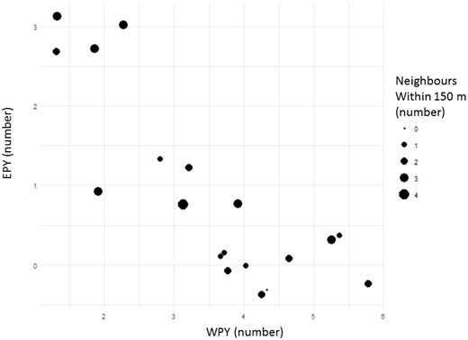
The number of WPY and EPY in 19 nightingale nests. The circle size represents the number of neighbors within 150 m. Nests with very high proportions of EPY (upper left corner) were all situated in densely populated areas (at least two neighbors within a 150 m radius). Although nests with relatively high numbers of neighbors may also reach high proportions of WPY, the more isolated nests (no or only one neighbor within a 150-m radius) predominate here. P = 0.009 (GLM, see Table 1 for details). (Note: circle positions are slightly jittered to ensure visibility of all circles).
Overview on results from generalized linear model
| Response variable | Predictor variables | Estimate | SE | df | t/z | P |
|---|---|---|---|---|---|---|
| WPY and EPY/nest | Age | −3.18 | 1.71 | 17 | 1.86 | 0.063 |
| Pairing date | −0.13 | 0.11 | 17 | 1.23 | 0.218 | |
| Buzz repertoire size | −0.06 | 0.29 | 17 | −0.2 | 0.844 | |
| Repertoire size | 0.06 | 0.03 | 17 | 1.98 | 0.048 | |
| Neighbors within 150 m | −1.39 | 0.53 | 17 | 2.63 | 0.009 |
Notes: As response variable we used the binary outcome of being either WPY or EPY for each chick in each nest. Within nests of social fathers, the odds for EPYs was reduced by 6% by a one-unit increase in repertoire size and is increased by 25% by one more neighbor (mean number of neighbors: 1.8 ± 1.02; range: 0–3) which was obtained from exposing the estimate given in the table. n = 19.
The relation between EPP and repertoire size in more detail
Repertoire sizes varied strongly between males under study, ranging from 113 to 243 different song types (171.5 ± 32.5; mean ± SD). Repertoire sizes of social fathers who suffered from cuckoldry were not different from those of social fathers who had not been cuckolded (Mann–Whitney U test; U = 54, P = 0.94; Figure 2). However, pairwise comparison of repertoire sizes of social and extrapair mates within single broods revealed a trend that extrapair males had larger repertoires (signed Wilcoxon test, n = 8; Z = −1.85, P = 0.08; Figure 3).
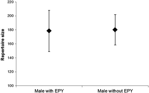
Repertoire size (means ± SD) of social mates with and without EPY in their nests. No difference was detected between groups of males. See text for statistics.
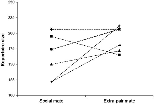
Pairwise comparison (n = 8) of repertoire sizes of social (n = 6) versus extrapair mates (n = 6) within single broods. Shown are repertoire sizes of single males (two social mates shared paternity with two different extrapair mates, and two extrapair mates fathered EPY in different nests, i.e., these males entered twice). In six cases (out of eight) extrapair mates had larger repertoires. See text for statistics.
Discussion
We assigned fatherhood within 28 broods of common nightingales in order to study the extrapair mating behavior of this socially monogamous songbird species with complex song. The average EPP rate was 21.5% of all offspring analyzed. Different from many other studies, we were able to not only distinguish EPY from WPYs within nests, but were also able to determine the identity of extrapair fathers for almost all chicks. This allowed us to inquire into factors being predictive for EPPs. With neighbor settling patterns and song repertoire size we did indeed identify two features that were related to the proportion of EPP.
The average EPP rate of 21.5% is close to the average EPP rate observed in other passerines (17% based on a comparison of 73 species; reviewed in Wink and Dyrcz 1999). However, it is higher than the average rate in socially monogamous bird species being 11.1% of offspring (reviewed in Griffith et al. 2002). Compared with other members of the Muscicapidae family it is in the upper range of the species investigated (reviewed in Hasselquist and Sherman 2001,). In general, it is expected that extrapair rates are low to moderate in species that do not show pronounced sexual dimorphisms (reviewed in Møller and Birkhead 1994) but high levels of paternal care (reviewed in Møller 2000) such as the nightingale. In these species, females are expected to base their choice primarily on direct fitness benefits such as male contribution to parental care. These predictions seemed initially confirmed by results of a preliminary study on nightingale paternity reported by Amrhein (unpublished data PhD thesis 2004) indicating low rates of EPP in the population under study (average EPP rate of 7.5% obtained from paternity analyses across 6 years from 1998 to 2003; 147 offspring in 39 broods). By contrast, we found that in our study population EPP occurs more often than expected by these predictions and prior results. Thus, the nightingale is among the species where EPP proportions differ considerably between populations (reviewed in Westneat and Sherman 1997). At the same time, EPP rates might differ across years within the same population as it has been shown for the closely related blue throat Luscinia svecica (Johnsen and Lifjeld 2003). This suggests that it is worth following EPP patterns both over a longer timeframe and within different populations.
Population density has been suggested as one explanation of within-species differences in EPP rates (Westneat et al. 1990) and our results support this notion. We found that in our population territorial settlement of males strongly influenced the occurrence of EPP. Since we were able to assign paternity of chicks almost exclusively to males belonging to the population, we can exclude the possibility that EPY were sired by non-territorial floaters. For the majority of nests that contained EPY, one or two neighboring males (either direct or close-by neighbor) were identified as genetic fathers of EPY, whereas in only very few cases EPYs were sired by a more distant male. Considering this pattern in more detail, we found that males that settled in “hot spots” with two or more close neighbors within a 150 m radius were more likely to have EPY within their nests. Our results indicate the importance of the availability of potential extrapair mates in relative proximity also for nightingales and suggest that not only overall population density, but also settling patterns (“clumped” vs. “further-spaced” territories) might affect EPP rates. From the perspective of individual males, it might still pay off to breed in close proximity to others when advantages to sire EPYs outweigh the costs of suffering from EPYs or considering other factors favoring a clumped distribution of territories (such as, e.g., food abundance). Generally, females or males that have to invest in longer forays to engage in EPCs may suffer from costs that come with seeking for extrapair mates such as desertion by the social mate or less paternal investment (female costs) and paternity loss in own nest (male costs). Instead nightingales may engage in EPCs only when conditions favor extrapair mating opportunities and when benefits (i.e., mating with higher quality males to increase offspring fitness or mate with more females to increase reproductive success) are expected to be high.
Besides male settlement pattern, our study provides first evidence that male song, namely repertoire size, is related to extrapair mating behavior in nightingales: a multivariate generalized linear model did show that social mates with larger repertoires were less likely to have EPY in their nest. In more detail, when all other influencing factors were hold at a constant level, a one-unit increase in repertoire size (just one more song in the repertoire) would reduce the probability of being cuckolded by 6%. Considering the large differences in individual male repertoire sizes this underlines the potential of repertoire size to be an indicator of signal of male quality in this species. Large-repertoire males might either be able to better mate-guard their females; or females of small-repertoire males might be able to circumvent mate-guarding and/or seek EPC with males having larger repertoires than their own mate. When we directly compared repertoire sizes of social mates who suffered from cuckoldry (i.e., had at least one EPY in their nest) versus repertoires sizes of social mates who did not have EPY there was no difference in male repertoire size. This can be taken as a hint that within social pairs of nightingales a male’s repertoire size (alone) does not prevent a male from losing paternity in own nests (social mate’s perspective), and that other male traits and/or song characteristics might additionally affect extrapair mating behavior within social bonds (e.g., Naguib et al. 2001; Kunc et al. 2006; Schmidt et al. 2008; Sprau et al 2013; Bartsch et al. 2015a). Yet, comparing repertoire sizes of social and extrapair mates of single broods revealed that extrapair males tended to have larger repertoires. Although this finding needs to be interpreted cautiously given the small data set (repertoire comparison of eight pairs of males), repertoire size might have an impact on which males are finally successful in obtaining EPP (extrapair mate’s perspective). Assuming that females initiate EPCs (by among others paying attention to song repertoires), their choice might be based on the relative evaluation of their social and potential extrapair mates’ song features. Although not specifically shown for song repertoires, similar results have been obtained for example in great tits and black-capped chickadees where females were either more likely to visit neighboring males or have been found to engage in EPCs depending on their social mates’ performance in male vocal interactions (Otter et al. 1999; Mennill et al. 2002). For nightingales it is also known that females pay attention to male vocal interactions and respond to differences in the song patterning of interacting males (indicating preferences for certain performance roles; Bartsch et al. 2014).
The role of repertoires in mate choice has been intensively studied assuming that large repertoires serve as an indicator for male quality (i.e., superior genetic constitution, reviewed in Nowicki et al. 2002) and that female choose large repertoire males to increase offspring fitness (e.g., McGregor et al. 1981; Gil and Slater 2000; Reid et al. 2005). However, only few prominent studies showed that females indeed base their choice on repertoires (reviewed in Byers and Kroodsma 2009) and evidence for an effect of repertoire size in extrapair mating decisions is extremely rare (reviewed in Garamszegi and Møller 2004). Generally, we have only very limited knowledge on how male song shapes extrapair mating decisions in different species (studies showing a relationship between song and EPP: Hasselquist et al. 1996; Kempenaers et al. 1997; Forstmeier et al. 2002; Byers 2007; studies finding no effect of song: e.g., Buchanan and Catchpole 2000; Forstmeier and Leisler 2004; Marshall et al. 2007; Hill et al. 2011). Against this background our studies provide valuable data on how certain song parameters (in combination with other factors) might influence EPP in natural populations.
To conclude, the engagement in EPCs in nightingales seems to be influenced by several factors including settlement patterns as ecologically based factor and male song as an indicator for male quality. As a result, EPP rates may vary within a population and across populations. We suggest interpreting our findings as a hint on a flexible mating strategy that might vary between individuals, years, and/or populations of nightingales. Still, we are just at the beginning to understand extrapair mating decisions in nightingales and songbirds in general. In order to fully understand the evolution of EPP in socially monogamous species with elaborate song, genetic paternity analyses need to go hand in hand with detailed behavioral studies (i.e., on foray patterns of individuals during the fertile period) and thorough analyses of male song.
Experimental Ethics
We followed the Guidelines for the Use of Animals in Research and methods complied with current laws of Germany. Bird banding was granted by the Landesumweltamt Brandenburg on behalf of the Vogelwarte Hiddensee.
Author Contributions
C.L. and S.K. designed the study, C.L. collected all data in the field and analyzed the genetic material, C.L. and S.K. did the song analyses, K.W. and J.W. supervised C.L. in laboratory work on paternity analyses, M.W. and C.L. did the statistical analyses, C.L. and S.K. wrote the manuscript.
Acknowledgements
We are thankful to Dagmar Thierer, Arpik Nshdejan, and Iris Adam for their help during laboratory work, and to numerous students for assistance in the field. Also, we thank Hansjörg Kunc and Marc Naguib for their advice and valuable comments on the manuscript. We thank Sarah Benhaiem for statistical advice. C.L. was funded by Berlin Funding for Graduates (Elsa-Neumann-Stipendium des Landes Berlin). We followed the Guidelines for the use of Animals in Research (compliance with the current laws of Germany) and bird banding was granted by the Landesumweltamt Brandenburg on behalf of the Vogelwarte Hiddensee.
Funding
CL was supported by the Elsa-von-Neumann foundation who granted a PhD scholarship.
References
Appendix
General remarks on CERVUS output
The set of microsatellite loci used in the paternity analysis yielded in a high average combined exclusionary power for paternity (1st parent = 0.99900481, 2nd parent = 0.99997553). Likewise, the polymorphic information content (PIC) averaged across all loci was high (0.73) with individual PICs ranging between 0.40 and 0.94 (see Appendix Table A3).
However, results on Hardy–Weinberg equilibrium calculations revealed that 6 out of 10 loci typed significantly departed from Hardy–Weinberg equilibrium, that is, in these cases expected genotype frequencies did not match observed frequencies. This indicates that we were not able to type all loci correctly as our data set contained either more homozygous (LM26, LM34, LM43, LM44, HrU6) or more heterozygous (Mcy4) allele combinations than expected. Several authors have dealt with genotyping errors (like increased homozygosity) and give possible explanations for this phenomenon including biological reasons as well as failures during laboratory work (e.g., Pompanon et al. 2005; Dakin and Avise 2004; Oosterhout et al. 2004; Kalinowski et al. 2007). We nevertheless decided to include all loci in our analysis for the following reasons: the set of loci yielded in a high average combined exclusionary power for paternity and likewise, the PIC averaged across all loci was high (see above) indicating that our data set reached sufficient statistical power. Additionally, in most cases of assigned paternity the social father or a close neighbor was identified as genetic father, which further indicates that the real father instead of any random male was most probably assigned.
Overview on data sampling and results of paternity analysis across four breeding seasons
| Nests (or social | Nests completely | Nests | Offspring | ||||
|---|---|---|---|---|---|---|---|
| fathers) entering | sampled and | containing | Offspring | sampled and | |||
| Year | Nests | GLM | genotyped | EPY | total | genotyped | EPY |
| 2009 | 4 | 2 | 3 (75%) | 3 (75%)1 | 18 | 17 | 3 (18%)3 |
| 2010 | 8 | 8 | 6 (75%) | 6 (75%)1 | 38 | 36 | 12 (33%)3 |
| 2011 | 15 | 9 | 11 (73%) | 4 (27%)1 | 68 | 63 | 11 (18%)3 |
| 2012 | 1 | 0 | 1 (100%) | 0 (0%)1 | 5 | 5 | 0 (0%)3 |
| N | 28 | 19 | 21 (75%) | 13 (46%)1 | 129 | 121 (95%)2 | 26 (22%)3 |
aCalculated from the total number of nests investigated.
bPaternity has not been assigned for eight chicks (four chicks without blood sample, four chicks not assigned by the program).
cCalculated from the number of offspring sampled and genotyped.
Characterization of microsatellite loci in the nightingale
| Multi-plex | Locus | U/μL | Primersequence (5′–3′) | Anneal.temp. (°C) | Observed allele size range (bp) | |
|---|---|---|---|---|---|---|
| 1 | LM3 | 0.089 | (F) CCA GGG CTG AGA TCC CAG AGC ATC T | 65 | 173–498 | |
| (B) TGG CTT TTC CCA TTC CTC ATT TCC C | ||||||
| 1 | LM6 | 0.222 | (F) TTG GCA AGT CAG TCA AGG CTG AGG T | 90–116 | ||
| (B) CTG TGG CAC TGT GTG CTG TGG GTT T | ||||||
| 1 | LM26 | 0.666 | (F) GCA TTA AAG GCA ATA GAC ATT GTG T | 181–200 | ||
| (B) AAA ATA CTC TTG AGG GTG TGG TAT G | ||||||
| 2 | LM34 | 0.139 | (F) AGC CCA AGG TGT GCT TCC TG | 60 | 194–267 | |
| (B) GGG GCA AAG ACC ACG TAA CC | ||||||
| 2 | LM37 | 0.139 | (F) CAA CTT GTC CCT GGA ACC AG | 214–226 | ||
| (B) ACC TGA GCA TTG CAC AGA GC | ||||||
| 2 | LM43 | 0.278 | (F) GTA CAG GGA TTG CGC TTG TC | 316–394 | ||
| (B) CAG TGC ATA GTC TCC GTG G | ||||||
| 2 | LM45 | 0.444 | (F) GGA ACC ATG GCG CCA AGC | 189–226 | ||
| (B) GAG TCA GCC GTG CCG AGC | ||||||
| 3 | HrU6 | 0.500 | (F) GCT GTG TCA TTT CTA CAT GAG | 49 | 162–261 | |
| (B) ACA GGG CAG TGT TAC TCT CC | ||||||
| 3 | Mcy4 | 0.500 | (F) ATA AGA TGA CTA AGG TCT CTG GTG | 154–171 | ||
| (B) TAG CAA TTG TCT ATC ATG GTT TG | ||||||
| 4 | LM44 | 1.000 | (F) CCG TAT GCA GCC AGG ATC | 65 | 210–264 | |
| (B) GAT ACC AGA GGT CTC TTA C | ||||||
Characterization of microsatellite loci in the nightingale adopted from Cervus 3.0 output allele frequency analysis
| Locus | K | N | HO | HE | PIC | HW | FNull |
|---|---|---|---|---|---|---|---|
| LM3 | 30 | 190 | 0.926 | 0.900 | 0.890 | NS | −0.0175 |
| LM6 | 9 | 190 | 0.847 | 0.792 | 0.759 | NS | −0.0376 |
| LM26 | 8 | 185 | 0.405 | 0.542 | 0.489 | *** | +0.1603 |
| LM34 | 9 | 190 | 0.379 | 0.651 | 0.611 | *** | +0.2753 |
| LM37 | 8 | 189 | 0.730 | 0.692 | 0.638 | NS | −0.0303 |
| LM43 | 29 | 189 | 0.831 | 0.931 | 0.924 | ND | +0.0555 |
| LM44 | 12 | 186 | 0.570 | 0.784 | 0.753 | *** | +0.1596 |
| LM45 | 13 | 190 | 0.826 | 0.826 | 0.804 | NS | −0.0003 |
| Mcy4 | 6 | 187 | 0.706 | 0.587 | 0.520 | ** | −0.1063 |
| HrU6 | 32 | 179 | 0.944 | 0.955 | 0.951 | ND | +0.0039 |
Notes: Calculations are based on 190 individuals (125 offspring, 65 males). Number of alleles (k), individuals typed (N), observed and expected heterozygosity (HO and HE), PIC, Hardy–Weinberg equilibrium (HW), and frequency of null alleles (FNull).

