Quantifying Fertilizer Application Response Variability with VHR Satellite NDVI Time Series in a Rainfed Smallholder Cropping System of Mali

Abstract

Soil fertility in smallholder farming areas is known to vary strongly on multiple scales. This study measures the sensitivity of the recorded satellite signal to on-farm soil fertility treatments applied to five crop types, and quantifies this fertilization effect with respect to within-field variation, between-field variation and field position in the catena. Plant growth was assessed in 5–6 plots per field in 48 fields located in the Sudano-Sahelian agro-ecological zone of southeastern Mali. A unique series of Very High Resolution (VHR) satellite and Unmanned Aerial Vehicle (UAV) images were used to calculate the Normalized Difference Vegetation Index (NDVI). In this experiment, for half of the fields at least 50% of the NDVI variance within a field was due to fertilization. Moreover, the sensitivity of NDVI to fertilizer application was crop-dependent and varied through the season, with optima at the end of August for peanut and cotton and early October for sorghum and maize. The influence of fertilizer on NDVI was comparatively small at the landscape scale (up to 35% of total variation), relative to the influence of other components of variation such as field management and catena position. The NDVI response could only partially be benchmarked against a fertilization reference within the field. We conclude that comparisons of the spatial and temporal responses of NDVI, with respect to fertilization and crop management, requires a stratification of soil catena-related crop growth conditions at the landscape scale.

1. Introduction

The demographic explosion of sub-Saharan Africa presents significant challenges for food production, which cannot be achieved without agricultural intensification [1]. Smallholder systems are characterized by enormous yield gaps [2], which may be reduced through integrated soil fertility management, improved crop-livestock integration, multi-purpose crops, and other sustainable intensification practices [3]. These options will, however, be implemented in an evolving socio-economic and climatic context where multiple drivers of change may increase exposure to risk, alter patterns of vulnerability, and open opportunities for agricultural development, especially through changes in urban demand, market access, IT penetration, and social differentiation [4]. The huge variability in farming and cropping practices [5] and returns on investments already observed today [6] is therefore likely to exacerbate in the future. Higher dependency on information may entail additional risk for smallholders and other agricultural stakeholders, notably in the presence of information asymmetries.

Monitoring changes in productivity across scales is a daunting challenge indeed in heterogeneous smallholder systems, for example in Mali’s cotton belt. In this area, with an increasing land shortage and reduced options for fallows [7], farmers rotate crops and apply manure, crop residues, household waste and compost to manage soil fertility in increasingly fragmented fields (currently 1.4 ha on average). Inorganic NPK fertilizer is commonly applied to cotton and maize in moderate quantities, but overall low organic matter content and nutrient deficiencies prevail. Catenary variation in soil properties is well known to farmers [8], and hence determines in part land management practices and observed spatial cropping patterns across the landscape. Field position on the topo-sequence influences soil fertility management [9], crop types and rotations [10], agro-biodiversity management [11] and agro-forestry practices [12]. However, this seemingly clear-cut relationship of soil characteristics with landscape position is obscured by farm management, the complex superposition of farm-centered management rings [13], by unequal farmer endowment and resource use [14], and by several other abiotic and biotic factors of random variability [15].

Fortunately, modern information technologies including remote sensing can help to monitor crop performance at levels of granularity increasingly compatible with smallholder farming [16]. This may open practical support applications for precision agriculture, allowing the exploitation, rather than the mitigation, of spatial heterogeneity, and the demonstration that increased productivity and enhanced livelihoods are not necessarily antithetical with complex cropping systems, and may actually thrive on the latter.

This study focuses on the analysis of remote sensing’s potential to retrieve crop status information at sub-field scales in heterogeneous smallholder rainfed production systems. The objective of the paper is to measure the sensitivity of the NDVI signal to on-farm fertility treatments applied to five locally important crops: cotton (Gossypium sp.), pearl millet (Pennisetum glaucum (L.) R. Br.), sorghum (Sorghum bicolor (L.) Moench), maize (Zea mays L. ssp.), and peanut (Arachis hypogaea L.). These five crops represent over 84% of the harvested area in Mali’s old cotton basin [17]. NDVI sensitivity to fertilizer applications was first analyzed at the field scale. For each crop, the amplitude and period of strongest plant response to fertilization is discussed. The spatial variance components were quantified with respect to the effects of fertilization and to within and between field variability associated with management, soil characteristics and catena position in the landscape.

2. Data Acquisition and Processing

As part of the STARS project [18] (Spurring a Transformation for Agriculture through Remote Sensing) an intensive coordinated ground and remote sensing campaign ran during the 2014 and 2015 growing seasons in the Koutiala District (Mali) and the Bebeji Local Government Area (Nigeria). The aim was to assess the performance of remote sensing (RS) imagery for crop monitoring in smallholder farming systems. Remote sensing data acquisitions and analyses involved both VHR satellite and UAV imagery. A set of variables was concurrently collected in-situ, following a standardized protocol [19] for both sites, and synchronous with bi-weekly UAV and (cloud cover permitting) satellite data acquisitions. This paper reports on data collected in the Koutiala district (Mali) in 2014.

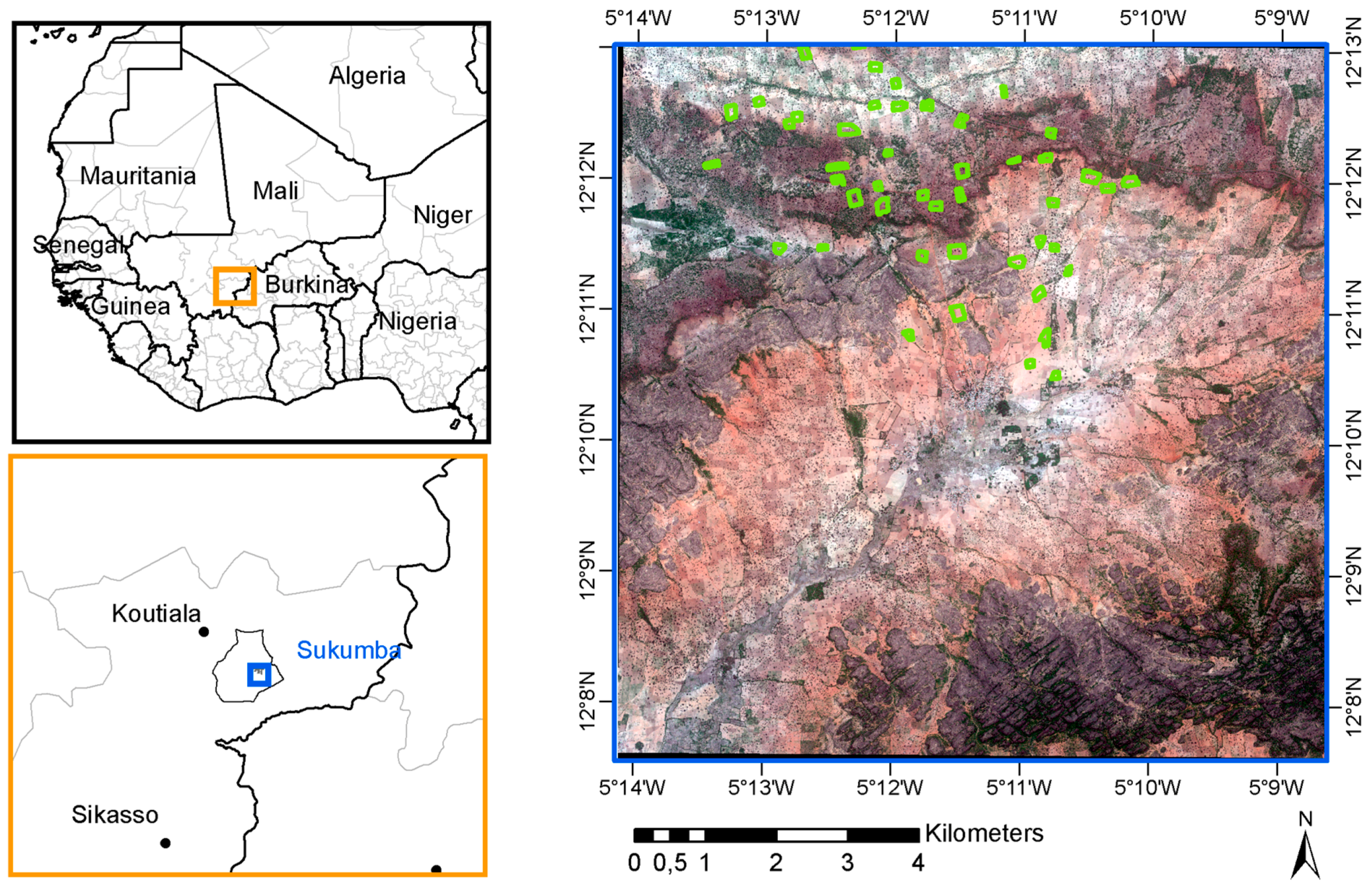
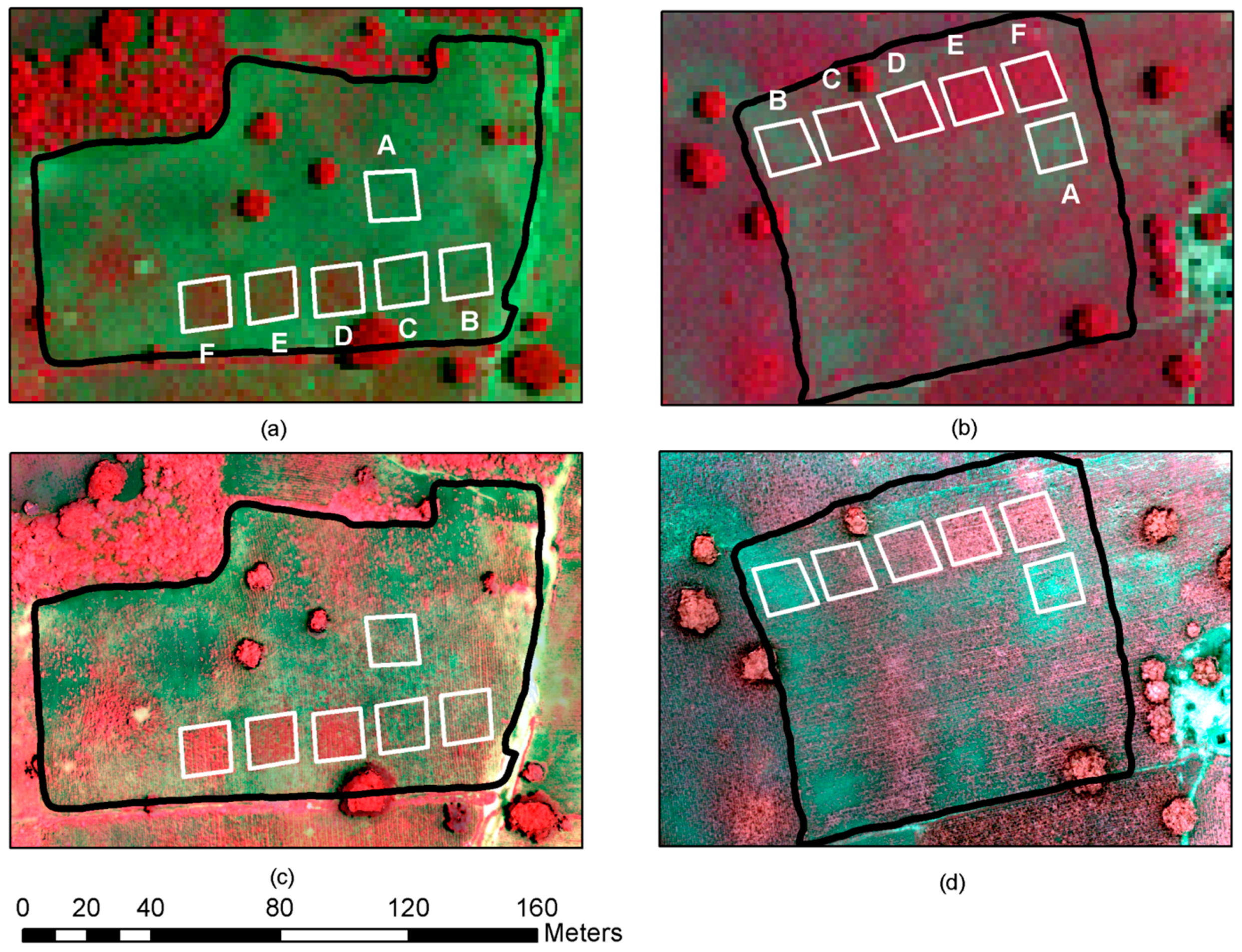
2.1. Study Area, Near Sukumba, Mali

The study area is situated within the terroir of the Sukumba community (commune of Koningue, Koutiala District, Sikasso Region) in the southeastern part of Mali located in the Soudano-Sahelian region (Figure 1) where rainfed cropping is the common practice. Forty-eight farmer fields were selected to host fertility treatments, sampling a topo-sequence from alluvial lowlands (altitude of 350 m above sea level) to the top of the plateau, with slopes characterized by breaks with locally steep inclines (total elevation difference of about 50 m). The catena ranges from deep, moderately fine textured and relatively well-drained soils in the lowlands (Plinthic/Ultic Haplustalfs, Oxic Haplustults) to moderately deep to shallow, gravelly and lateritic soils in the midslopes (Typic Cuirustalfs, Mollic Cuirorthents, Lithic Haplustalfs), and again to moderately deep, argillic soils on the plateaus [20]. Soil surface color markedly varies from reddish in sloping sections to light grey in flatter areas such as plains and plateaus (Figure 1).

2.2. VHR Satellite Series

A dataset of 15 images was acquired by the Digital Globe (DG) satellite constellation during the 2014 growing season over a 10 km × 10 km area centered on the Sukumba village (

Table 1. Available Digital Globe images series acquired over the Sukumba site, Mali in 2014 including GeoEye1 (GE01), WorldView2 (WV02) and QuickBird2 (QB02). The right column (Correction Method) refers to the specific type of processing applied to the images as described below.

Acquisition Date	Satellite	Product Level	Product Type	DEM Correction	Correction Method
1 May 2014	GE01	LV2A	Standard	Coarse DEM	4
22 May 2014	WV02	LV3D	Orthorectified	Fine DEM	4
30 May 2014	WV02	LV3D	Orthorectified	Fine DEM	4
18 June 2014	QB02	LV2A	Ortho ready	Base Elevation	2
24 June 2014	GE01	LV3D	Orthorectified	Fine DEM	4
26 June 2014	WV02	LV2A	Ortho ready	Base Elevation	2
8 July 2014	GE01	LV2A	Standard	Coarse DEM	4
11 July 2014	QB02	LV2A	Ortho ready	Base Elevation	2
29 July 2014	WV02	LV2A	Ortho ready	Base Elevation	2
7 August 2014	GE01	LV3D	Orthorectified	Fine DEM	4
26 August 2014	GE01	LV2A	Standard	Coarse DEM	3
4 October 2014	QB02	LV2A	Standard	Coarse DEM	3
18 October 2014	WV02	LV2A	Ortho ready	Base Elevation	1
1 November 2014	WV02	LV2A	Ortho ready	Base Elevation	1
14 November 2014	WV02	LV2A	Ortho ready	Base Elevation	1

). The spatial resolution of these images varies from 0.5 m to 0.61 m for the panchromatic band and from 2 m to 2.44 m for the multispectral bands. This constitutes an unprecedented dataset for Sudano-Sahelian smallholder agriculture.

In order to ensure accurate imagery geo-location in a landscape characterized by relatively few artificial man-made structures, a set of 65 Ground Control Points (GCP) was used. Some GCPs were located on rock outcrops but most GCPs were concrete structures with a standard cross shape (width: 120 cm; thickness: 20 cm). All GCPs were painted white around mid-August of 2014. They are easily identified on satellite images while they were initially designed for the georeferencing of images acquired by a UAV operating only in the Northern part of the 10 km × 10 km study area (cf. Section 2.4). Additional GCPs corresponding to fence or hedge corners were identified in the Southern part of the study area. The geographic coordinates of GCPs were recorded with a differential GPS system with centimeter accuracy.

The complete set of GCPs covering the entire study area is only visible on images acquired after mid-August. Moreover, various processing levels have been applied by DG on the time series; some were orthorectified (the so-called Standard and Orthorectified product types), while others were not (Ortho ready product type). Therefore, combining these two constrains, four dedicated geometric correction approaches were used to ensure that the time series were geometrically consistent. The four correction methods as reported in Table 1 are:

• Ortho ready DG-products with no DEM correction by DG (base elevation) were orthorectified using SRTM 30 m DEM and GCPs when available, i.e., after 26 August 2014. Out of the total set of 65 GCPs, a subset of 38 GCPs was used to correct the 18 October 2014 image. Orthorectification resulted in a geometric accuracy of 0.84 m (RMSE), assessed on remaining GCPs not used for orthorectification. This image was thereafter taken as master image to geometrically correct the other images in the absence of GCPs (methods 2 and 4 in Table 1). The same set of GCPs was used to orthorectify the 3 last ortho ready standard images of the series using the same method.
• Ortho ready DG-products acquired before 26 August 2014 were first orthorectified with the SRTM 30 m DEM without any GCP, and were subsequently co-registered to the master image (i.e., 18 October 2014 image orthorectified with the first method as describe here above) thanks to an automatic image-to-image registration algorithm providing 25 tie-points well distributed over the image.
• Products orthorectified by DG are of two types: standard product orthorectified using a coarse DEM (SRTM 90 m) and orthorectified product pre-processed by DG with fine DEM (SRTM 30 m). Both product types were simply georeferenced with the set of 38 GCPs for dates after 26 August 2014.
• Products orthorectified by DG (both standard product and orthorectified product types) acquired before 26 August 2014 were georeferenced using the master image by automatic image-to-image registration (as mentioned above for case 2).

Orthorectified image DNs were then converted to top-of-atmosphere reflectance [21,22]. Clouds and cloud shadows were detected using an unsupervised classification and then the areas where masked out. All the processing methods resampled the images at a 2 m pixel size using the nearest neighbor algorithm. GCPs were visualized first on panchromatic images (to increase the precision), and then applied to the multi-spectral images.

2.3. In-Situ Data Collection

2.3.1. Soil Fertility Trials

Cropping systems in the Koutiala district are based on cotton, maize, sorghum, and millet rotations. The five main crop types that were covered by the field campaign also included peanuts. Under rainfed conditions, the growing season ranges from late May to November. A set of 48 farmer fields was selected to monitor plant growth and development during the 2014 growing season. To cover the wide range of within-season variation that may be encountered in these heterogeneous environments, suitable fields (farming management units) were identified through a participatory selection process along the catena to adequately sample gradients in soil physical and chemical properties. Within each farmer field monitored, fertility treatment plots were included to ensure a full range of variability that may be present in the local landscape. A standardized protocol [19] with recommended fertilizer type and quantity for each crop type was used (

Table 2. Fertility levels (kg/ha) for each plots of each crop type (five plots (B; F) for millet and sorghum field; four plots (B; E) for maize, peanuts, and cotton). DAP stands for Di-Ammonium Phosphate with 18% N, 46% P₂O₅ and 0% K₂O; “15-15-15”, locally called ”complexe céréales” is also a NPK fertilizer with 15% N, 15% P₂O₅ and 15% K₂O; “Coton complex”, locally called “complexe coton” is a NPKSB fertilizer with 14% N, 18% P₂O₅, 18% K₂O, 6% S, and 1% BO₃; Profeba is a compound organic fertilizer, locally called “sabunyuman” [23] containing cattle manure, poultry manure and 14% N, 5% P, and 1% K in addition to various other micronutrients; Urea contains 46% N.

Millet/Sorghum	DAP	15-15-15	Urea	Kg N/ha	Kg P/ha	Kg K/ha
B				0.0	0.0	0.0
C			50	23.0	0.0	0.0
D	75		50	36.5	15.1	0.0
E	150		50	50.0	30.1	0.0
F		150	50	45.5	9.8	18.7
Maize	DAP	15-15-15	Urea
B		100	150	84.0	6.5	12.5
C	100		150	87.0	20.1	0.0
D		200	300	168.0	13.1	24.9
E	200		300	174.0	40.1	0.0
Peanut	DAP
B				0.0	0.0	0.0
C	50			9.0	10.0	0.0
D	100			18.0	20.1	0.0
E	150			27.0	30.1	0.0
Cotton	Cotton Complex	Profeba	Urea
B				0.0	0.0	0.0
C	150		50	44.0	11.8	22.4
D	200		100	74.0	15.7	29.9
E	200	10,000	100	109.6	43.1	6.0

). Urea was applied at earing, and other fertilizers at sowing. The fertility experiment layout is schematized in Figure 2. Within each field, five (cotton, maize, and peanut) or six (millet and sorghum) plots of 15 m × 15 m were picketed (Figure 2: solid outline boxes). One plot, and the remainder of each field was managed as per farmer practice (Figure 2: dashed outline box). Plant growth, development, biomass and grain yields were measured in all plots. Each participating farm could contribute only one field. Small field sizes did not allow for replicates within a single field, but instead treatments were replicated (10 cotton, 10 maize, 10 millet, 9 peanut and 9 sorghum fields) across the landscape.

2.3.2. Crop Development

Within each plot, five 2 m × 2 m quadrats were used for bi-weekly ground-based monitoring of plant development and growth, synchronous with UAV image acquisitions. There are therefore, 25 quadrats (5 quadrats for each of the 5 plots) per field for cotton, maize, and peanut; and 30 quadrats (6 plots × 5 quadrats) for millet and sorghum. The 4 corners of each plot were semi-permanently picketed and their position recorded with a differential GPS with centimeter accuracy in order to measure the exact same location at each field visit. At each bi-weekly field visit, non-destructive measurements of crop status, BBCH phenological development stage [24], weed prevalence rate, plant height, and ground cover (GC) fraction were assessed for each 2 m × 2 m quadrat following standardized protocols [19] and recorded in dedicated data entry forms on smartphones.

The ground coverage (GC fraction) of the soil background by green plant material was estimated using vertical photographs. These were taken with a 35 mm lens camera mounted on a L-shaped, 3 m telescopic pole, from nadir view above the canopy. Images were processed using the CAN-EYE freeware [25] to determine GC fraction by an human interactive process classifying pixels into bare ground and green vegetation classes.

2.3.3. Farming Practices

Information concerning crop type and variety, soil texture, and agronomic practices (soil preparation, sowing, weeding, fertilization, harvesting, etc.) was recorded for each of the 48 fields. After harvest, farmers also provided the fresh weights of total aboveground biomass and reproductive parts (quantified, for example, in number of carts or bags) for the entire field.

2.4. UAV Data Acquisition and Processing

A SenseFly eBee with Canon S110NIR camera (R, G, NIR bands) was used to acquire image mosaics every two weeks (synchronously with field measurements) [26]. Flight plans were optimized to cover the 48 fields located in the Northern part of the study area (Figure 1) in 7 flights, with each flight surveying a cluster of fields. Image acquisition settings ensured a 70% lateral and 75% longitudinal overlap and a target pixel resolution of approximately 10 cm × 10 cm on the ground.

All the pictures of a given flight were acquired with the same camera settings optimized shortly before takeoff. The shutter speed was set to maximum, i.e., 1/2000; and the sensitivity (ISO) and focal length settings were adjusted in order to slightly under-expose the picture (avoiding any saturation in the images).

The Canon camera records images in a raw format (.CR2). They are first converted to TIF format using eMotion software. Then, AgiSOFT Photoscan Pro was used to generate a Digital Surface Model (DSM) and an orthomosaic. For accurate image geolocation, the set of 50 GCPs distributed throughout the entire area of the 7 clusters was used. These GCPs were manually geo-located for each image to ensure an accurate point cloud for DSM generation and geometric correction as required for image mosaicking.

3. Methods

In order to assess the sensitivity of the NDVI response to the fertilization, the methodology included four main steps. Firstly, the seasonal temporal NDVI profiles are presented for each crop type and fertilization levels. Secondly, for each crop type and acquisition date, the potential to detect the fertilization treatments at the field scale was analyzed. Thirdly, the relationships between NDVI and plant growth (e.g., GC Fraction and height) were assessed. Finally, per crop type effects of fertilization treatments were compared to variation within and between fields in relation to catena position, farming practices and the soil type.

3.1. Seasonal NDVI Profiles under Different Fertilizer Applications

We first graphically assess the overall impact of fertilization by extracting the NDVI response from plots observed in the VHR satellite images. The mean and standard deviation were computed per crop type for each fertilizer application (plot B to F) and from emergence to senescence. We discuss the fertilization effect with regard to landscape-scale variability.

3.2. Detection of Fertilizer Application Responses at the Field Scale

In order to quantify the fertilization effect with regard to the total NDVI variability within one field, the variance components are estimated using an ANOVA variance decomposition method. The variance is decomposed for each field at each date (from crop emergence to harvest) using as inputs all individual pixels falling within the limit of the monitored fertilization treatment plots B–E (B–F for millet and sorghum: Figure 2). For this method the determination coefficients (R²) of a linear model estimates the part of variance explained by the fertilization treatment with respect to the total variance, and thus measure the ability to discriminate fertilization treatments using NDVI. The R² distribution among fields of a given crop type informs about the possibilities to assess fertility levels in relation to a reference plot within the same field. A higher median R² indicates a better discrimination of fertilization levels using NDVI for a given crop type at a given date. The R² distribution spread measures the consistency of the fertilizer application response between the different fields of a given crop type. R² values were marked as outliers when more than 1.5 times the interquartile range below quartile 1 or above quartile 3.

The normality of the residuals distribution has been verified. To validate the independency hypothesis, the spatial correlation is assessed using variograms of a UAV orthoimage acquired on 10 September 2014. Variograms were developed using the “gstat” add-on package available in the R software.

Additionally, given the non-linear plant response to fertilizer application, we identify the dose increment leading to the strongest reaction through a 2-by-2 comparison of NDVI means for each available dose increment. This was done for the (crop-specific) date of maximum fertilizer response. The date with the highest proportion of fields with a significant (t-test at p = 0.05) response to fertilization increments was defined as the date with the strongest effect of fertilizer application on crop NDVI response.

3.3. Relationships between Plant Growth Indicators and NDVI

Linear relationships between NDVI, ground coverage (GC) and plant height were established for each crop type separately using least-squares. Each observation for GC and plant height was a mean per plot. The NDVI was determined as the mean of all pixels within a plot. The 26 August 2014 image was selected as it corresponds to the period of maximum green biomass and for this date, in-situ data were also available. The image of 10 October 2014 was probably a better choice, as ground coverage was larger in that period for cotton, sorghum and millet but field data were not collected for these crops at this image acquisition date.

3.4. Detection of Crops Fertilization Treatment at Landscape Level

The NDVI response of a given crop type at a given date may also differ due to landscape position determining soil physical and chemical properties, agronomic management (including fertilizer application, sowing, weeding and harvesting dates) and thus plant growing conditions. Accounting for systematic variation in any of these factors can improve discrimination between fertilizer application amounts and other management practices. A hierarchical linear model was setup for each crop type to decompose the total NDVI variance to estimate the contribution of three components of variation: plot (induced by fertility treatment), field (mostly induced by other management factors) and landscape (mostly induced by environmental factors, including soil and elevation). The hierarchical model was selected, as fields are subordinate to strata while fertilizer application treatments were replicated in these fields. The average NDVI per plot was the dependent variable in the model. Therefore, a generalized linear model was fitted to the data, including all plots with treatments B–E (B–F for millet and sorghum), within the design matrix the categorical variables plot, stratum and fields. Fields factor was nested within the stratum. The GLM procedure in S.A.S. software (version 9.3) was used to fit the model with the statement “MODEL = plot, stratum, field (stratum)”.

The levels of the stratum effect were defined using expert knowledge on catena position (plateau, midslope, and lowlands), soil texture and drainage class. We expect that within a landscape stratum, soil types are reasonably similar and that farming practices are somewhat similar. The fields were selected in the landscape and fertility plots were repeated in each field (as described in the Section 2.3). All three factors were included as fixed terms in the model.

The larger the fraction of variance explained at the plot scale, the better fertilization application differences could be discriminated with NDVI for the considered crop type. If the strata effect explains an important part of the variance along with the plot effect, the NDVI of all the fields have to be compared within a given stratum (and not between strata) to discriminate fertilization application difference.

4. Results and Discussion

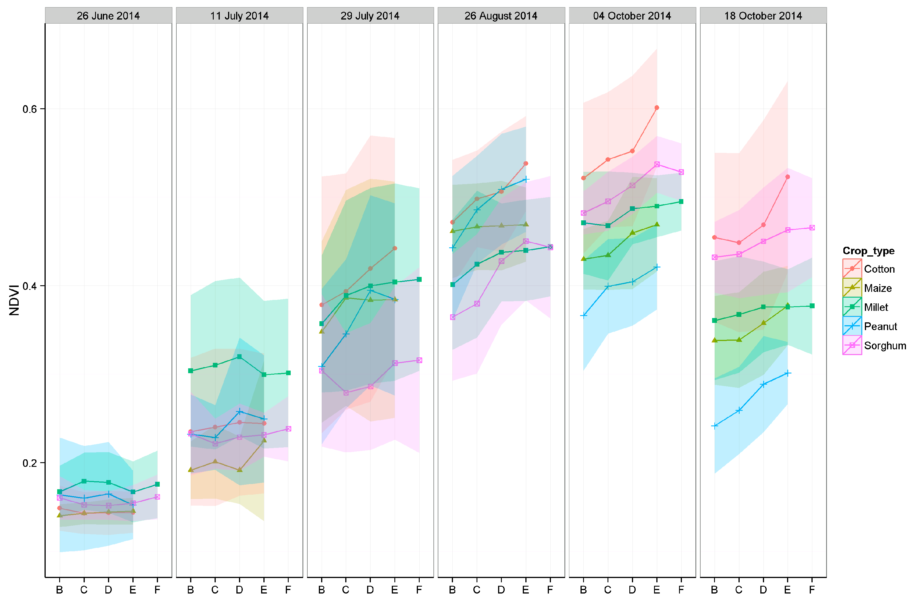
4.1. Seasonal NDVI Profiles under Different Fertilization Levels

Figure 3 shows the impact of fertilizer application treatments on NDVI for the five crops using six VHR images well distributed throughout the crop growing cycles and acquired after sowing. Millet NDVI is fastest to rise reflecting the vigorous establishment of the species. By late August differences between crops tend to reduce reflecting general canopy closure. Sorghum is the latest crop to establish with a delayed NDVI response. Sorghum showed a stronger NDVI increase with fertilizer applications than the other crops, clearly visible in late August. Millet displays an overall weak or no NDVI response to fertilizer application, as expected. Maize NDVI response to fertilizer is surprisingly weak throughout, indicated that ground cover was not strongly affected by the additional fertilizer applications. The highest apparent response to fertilizer application in early October is misleading and reflects differences in maize senescence. A fertilization effect is also observed for both cotton and peanut with the largest mean differences between plots on 4 October 2014 for cotton and 28 August 2014 for peanut.

However, standard deviations calculated for a given crop type and fertilization level reveal large differences between fields. The impact of fertilization on the NDVI, as observed for the five crops from about the end of August until the beginning of October, seems of comparable magnitude when compared to the background landscape-scale variability, as expressed by the large standard deviation. Detection of fertilization levels at landscape level will thus be impossible without taking into account other factors affecting NDVI.

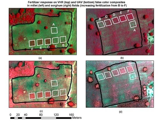
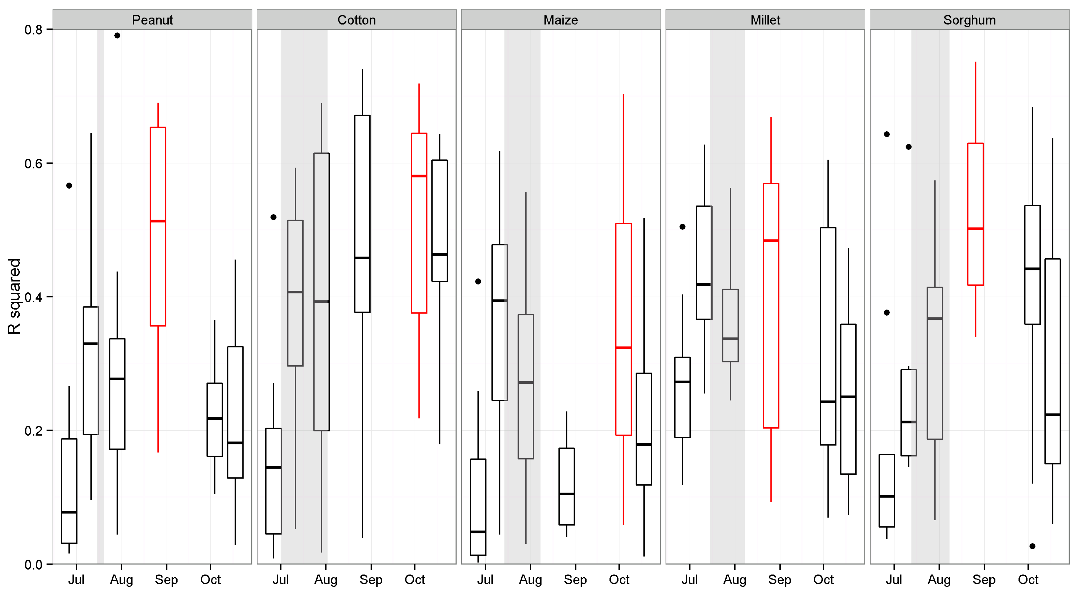
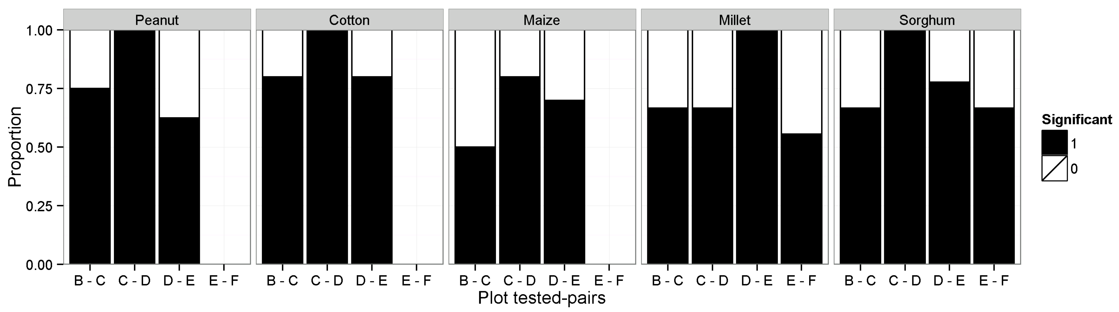
4.2. Detection of Fertilizer Applications at the Field Scale

Farmer fields in Sukumba are very heterogeneous and display a large NDVI variability, both between and within fields regardless of the typically small field sizes (1.4 ha on average). The effect of fertilizer can be observed visually in the field, and on both UAV and satellite images from about the end of August (Figure 4) until the beginning of October. In-situ observations highlighted important height and plant color differences between the most fertilized plots and the farmer’s practices (plots A). Figure 5 shows significant differences in the evolution of plant height and GC fraction between different plots of a millet and sorghum field (both crop types usually not fertilized by farmers). Both satellite and UAV detect gradual increase in NIR reflectance with fertilizer rates (Figure 4). However, the very large variability within and between the fields clearly shows that other environmental factors, such as residual soil fertility, presence of trees, decomposing tree root systems, anthills, termite mounds, etc. affecting plant emergence and subsequent plant growth, are important as well.

The regression model used to quantify the fertilization effect on the NDVI provides three major learnings (Figure 6). Firstly, the best period to observe a NDVI response to fertilization is crop specific: end of August for peanut, millet and sorghum fields and beginning of October for cotton. Maize also appears to respond more strongly in October, but that may be due to differential patterns of senescence. Most likely, this pattern may reflect variations in soil water holding capacity rather than a fertilizer response. Secondly, the 9–10 fields of each crop have very different responses to fertilization leading to a wide range of R² values. This suggests that the feasibility to detect differences in soil fertility at the landscape scale will be impeded by a very large between-field variance. This is a function of different management practices (such as sowing dates, occurrence of pests and diseases) and biophysical conditions. Among these, crop type differences in the evolution of the sensitivity of NDVI to fertilization are also important. The last learning is that the response to fertilizer application on maize fields was weaker than the other crops, and is most likely the consequence of the fertilization under farmer’s practices, which was not well controlled at the time of trial establishment, reducing crop response to additional fertilizer inputs. Some cotton and maize fields had already been fertilized by farmers at the time of plot establishment. The fertilization quantities prescribed by the protocol have thus been adapted but some over fertilization should have occurred in plot B for these two crops. This could also contribute to the high value of R² prior the fertilization treatment, in mid-July.

When NDVI response to fertilization is strongest, the regression model explained at least 50% of the variance between plots within a given field for about half of the fields, except for maize. Many factors can explain the remaining part of the within-field variation. For example, African smallholders actively maintain economically and culturally valuable tree species inside their field crops (especially rain-fed). Treatment plots were not very close to trees, however they remain exposed to competition for water and nutrients. They also largely benefit from tree and leaf litter nutrient deposit, although this varies with catena position [12]. Tree cutting leads to multi-annual, residual fertility hotspots as tree root systems decompose resulting in spectacular islands of dense crop canopy. Positive feedback loops locally amplify initial differences in nutrient inputs and organic matter contents by processes that further limit plant growth and input of organic matter into the soil, such as soil crusting and soil erosion [27].

The model used to quantify the effect of the fertilization on the NDVI relies on the assumption of independence of the observed areas (i.e., the DG pixels). Figure 7 shows semi-variograms based on the 10 September 2014 image when fields are at their maximum ground cover and thus feature lowest spatial autocorrelation during the growing season. Pixel values are only strongly correlated on short distances as indicated by the low nugget values and steep rise of semi-variance. Image values are more or less uncorrelated beyond 2 m for peanut, maize and sorghum fields. The influence of spatial correlation is present at larger distances for cotton and millet, but 75% of the variance is still captured within 2 m. Without accounting for the point spread function of the various instruments, the satellite multispectral pixels can be considered as mostly independent as they sample the ground at a 2 m resolution.

The overall NDVI response to fertilizer application does not mean that all differences in application amounts can be quantified accurately. It only shows that at least one of the treatments affected the NDVI response. The plant response to fertilizer application is non-linear, but the NDVI difference between treatment pairs was significant in most cases (for at least 70% of the fields, as seen in Figure 8) for the most discriminating images as indicated by the red boxplots in Figure 6. More specifically, treatments in C and D plots were discriminated in all for peanut, cotton and sorghum fields. The maize crop again shows a larger similarity in NDVI response between the treatments, leading to a lower proportion of plots with a significant difference. In contrast to the other crops, in millet fields, the NDVI discriminated plots D and E (i.e., doubling the DAP dose) best. For this crop, a higher fertilizer dose was required for a significant response of the canopy reflectance. However, in poor soil fertility environment, the largest difference in NDVI was expected for plots B and C, but the strongest response in Millet was surprisingly observed for plots D–E, while other crops C–D for other crops). This likely indicates a very strong response variability within fields.

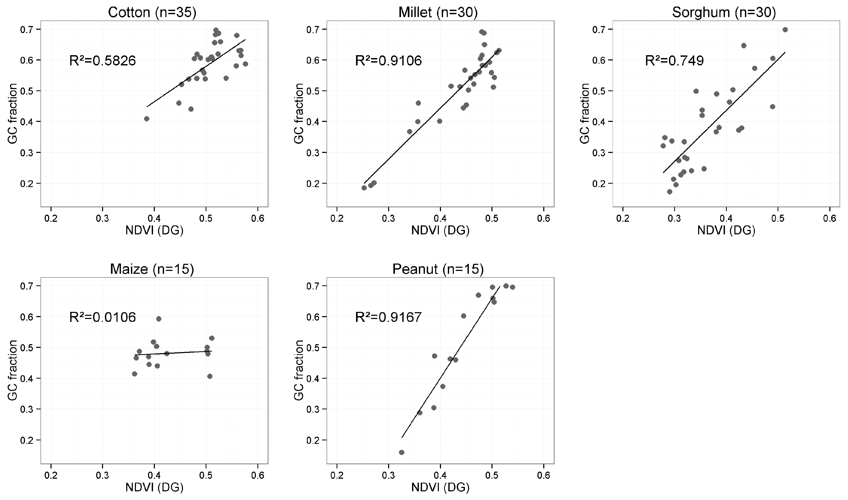
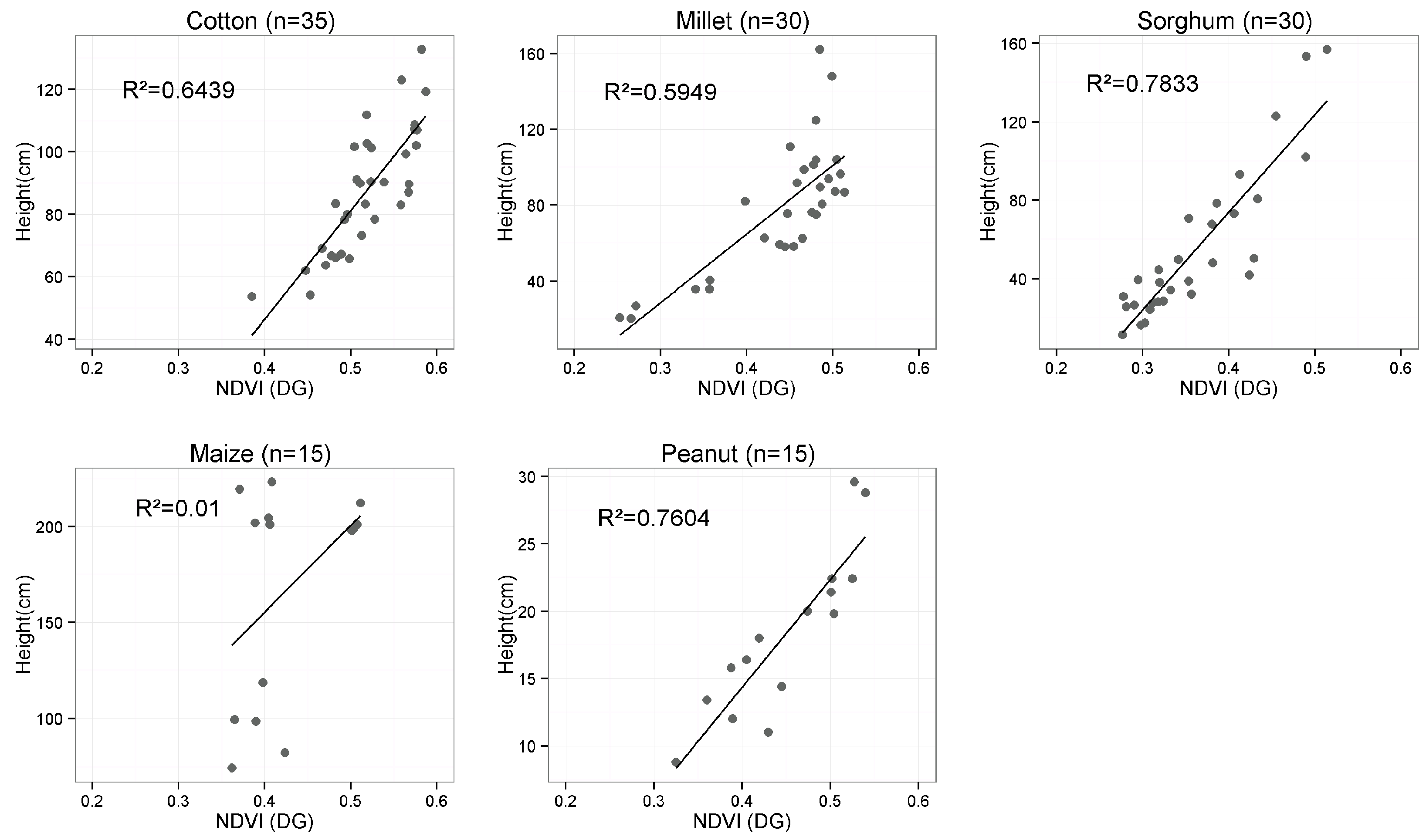
4.3. Relationships between Plant Growth Indicators and NDVI

Fertilization affects NDVI (as seen in Section 4.1) because plant growth strongly responds to fertilizer under nutrient limiting conditions. Figure 9 and Figure 10 show the relationships between NDVI and GC fraction or plant height, respectively. At the plot scale, NDVI was moderately to strongly correlated to GC fraction and plant height for cotton, millet, sorghum and peanut. A strong linear relationship was expected for peanuts between NDVI and GC fraction because of its plant canopy structure. Peanut growth leads to a small plant height increase but a strong ground coverage increase that directly impacts NDVI by masking the background soil surface. For maize, plant height did not respond strongly to fertilization. The range in GC fraction was very small for maize fields on 26 August 2014. In general, GC fraction is fairly low, even at more advanced growing stages due to large distances between rows and relatively low nutrient application levels.

4.4. Detection of Crops Fertilization Treatment at Landscape Level

The differences between the treatments in NDVI responses are significant when comparing plot-pairs of a given field and also when averaging over all fields. However, there is a large variation in response to fertilization treatment between individual fields. The hierarchical linear model described in Section 3.4 explains 75% to 95% of the total observed variance (Figure 11) when introducing the stratum and field effects. A large part of the explained variation in NDVI can be attributed to the differences between strata and between fields within a stratum due to interactions of soil type and field management. The fraction of variance explained by stratum and field factors was largest in the period between sowing (occurring within the period highlighted by a green color in Figure 11) and peak greenness (late August). NDVI differences due to different sowing dates were strongest at early growth stages but partly disappear during the growing season as the canopy closes.

The differences between fields within strata largely dominate the variance explanation for most of the crops. Between-field variability is well known in these heterogeneous environments and, the so-called outfields further away from the homestead usually have much lower yields and lower soil fertility than fields near the homestead [28] due to more organic nutrient inputs. A low fertility not only affects macronutrients such as N, P or K, but also micronutrients. Therefore, fertilizer response will be better on soils with high organic matter content as that is an indication of crop growth in recent years, reflecting larger micro-nutrient availability and absence of soil constraints including low pH or a large drought sensitivity [27]. Another significant factor of inter-field variability is labor constraints, relatively more acute during the peak demand at sowing and stemming from variable farm endowment levels, often correlated with farm sizes.

Within a stratum, relatively similar plant growth patterns were observed. Moreover, strata differ in their sensitivity to climate extremes, notably meteorological drought, due to distinct slope, potential rooting depth, texture, water holding capacity, runoff and drainage characteristics and, as a result differences in the amount of soil water that is available to plants. In case of early season dry spells or “false starts”, less favorable strata will observe more plant establishment failures leading to replanting and a delayed, more heterogeneous greening up of patches in this part of the landscape. This tends to maximize differences between strata early in the season (July), before all canopies are more fully developed including the re-planted patches [29].

The fraction of variance explained by fertilization treatment was generally small when compared to the variation due to field and stratum, ranging from 1% to 35% of the total variance observed. Its contribution to the explanatory power of the model was largest in early October for maize and sorghum fields and around the end of August for cotton and peanut fields (the high values observed for peanut in October were misleading as they correspond to fields already harvested). Sorghum responded strongly to fertilizer in its vegetative growth. As previously observed, Millet shows a weak response to fertilization treatment. This is partly related to more millet cultivation in the most constraining areas, reducing the fertilization effect in plots and increasing the contribution of the field effect. In addition, the fraction of variance explained by fertilization treatments would have been higher if farmers would not have fertilized some cotton and maize fields before the protocol had been put in place. Although total fertilizer application levels were adjusted proportionally to correct for that pre-existing situation, the effects of application on the control plots could not be corrected for.

5. Conclusions

Monitoring crop growth in spatially heterogeneous landscapes with trees in every field is very well possible with a time series of very high-resolution imagery. Large differences in temporal signatures between fields of a given crop type were observed. On average, crops clearly responded to fertilization, in terms of both crop height and ground coverage impacting the NDVI that is measured by a satellite sensor. NDVI differences between fertilizer treatments within individual fields were not consistent due to large within-field and within-plot variation, especially for treatments with a low fertilizer application (B and C).

The influence of fertilizer applications on crop NDVI response was proportionally small (lower than 35% of total variation) when compared to the influence of field management and catena position. Large differences in soil fertility and soil related constraints, interacting with plant density and field management, such as replanting at sub-field scale, mean that many factors influence crop growth and thus the NDVI response within a field. As a consequence, a measured NDVI response can only partially be benchmarked against a fertilization reference within the field. Indeed, the variance decomposition model applied at field level showed that 50% of the NDVI variance within a field is due to the fertilizer application for only half of the fields at times when the observed NDVI response was strongest. Moreover, the period with largest contrasts between treatments was crop specific: at the end of August for peanut and cotton and at early October for sorghum and maize. Standard precision agriculture methods based on comparisons of the response of a vegetation index within one field [30] are therefore not very useful. Accounting for other sources of variability in these heterogeneous landscapes is needed before such an approach can be applied.

However, at plot scale, strong relationships between NDVI and plant growth parameters including plant height and ground coverage were observed. This implies that NDVI imagery directly reflects differences in plant growth due to the inherent patterns of soil fertility and management. In the landscapes of southern Mali, differences in soils within the typical catena are large [12] and were strongly reflected in the responses of the five studied crops. We conclude that comparisons of spatial and temporal responses of vegetation indices for a particular crop type can only be done when plant growth conditions are similar, i.e., in within strata related to soil catena position in the landscape.

References

1. Godfray, H.C.; Garnett, T. Food security and sustainable intensification. Philos. Trans. R. Soc. Lond. B Biol. Sci. 2014, 369, 20120273. [Google Scholar] [CrossRef] [PubMed]
2. Van Ittersum, M.K.; Cassman, K.G.; Grassini, P.; Wolf, J.; Tittonell, P.; Hochman, Z. Yield gap analysis with local to global relevance—A review. Field Crops Res. 2013, 143, 4–17. [Google Scholar] [CrossRef]
3. Panel, T.M. Sustainable Intensification: A New Paradigm for African Agriculture; Imperial College London: London, UK, 2013. [Google Scholar]
4. Padgham, J.; Abubakari, A.; Ayivor, J.; Dietrich, K.; Fosu-Mensah, B.; Gordon, C.; Habtezion, S.; Lawson, E.; Mensah, A.; Nukpezah, D.; et al. Vulnerability and Adaptation to Climate Change in Semi-Arid Areas in West Africa: ASSAR Regional Diagnostic Study. Available online: https://www.weadapt.org/knowledge-base/assar/vulnerability-and-adaptation-to-climate-change-in-the-semi-arid-regions-of-east-africa (accessed on 20 June 2016).
5. Giller, K.E.; Tittonell, P.; Rufino, M.C.; van Wijk, M.T.; Zingore, S.; Mapfumo, P.; Adjei-Nsiah, S.; Herrero, M.; Chikowo, R.; Corbeels, M.; et al. Communicating complexity: Integrated assessment of trade-offs concerning soil fertility management within African farming systems to support innovation and development. Agric. Syst. 2011, 104, 191–203. [Google Scholar] [CrossRef]
6. Bielders, C.L.; Gérard, B. Millet response to microdose fertilization in south-western Niger: Effect of antecedent fertility management and environmental factors. Field Crops Res. 2015, 171, 165–175. [Google Scholar] [CrossRef]
7. Soumaré, M. Cotton-Based Cropping Systems Dynamics and Sustainability in MALI; Université Paris X Nanterre: Nanterre, France, 2008. [Google Scholar]
8. Gobin, A.; Campling, P.; Deckers, J.; Feyen, J. Integrated toposequence analyses to combine local and scientific knowledge systems. Geoderma 2000, 97, 103–123. [Google Scholar] [CrossRef]
9. Gandah, M.; Brouwer, J.; Hiernaux, P.; Van Duivenbooden, N. Fertility management and landscape position: Farmers’ use of nutrient sources in western Niger and possible improvements. Nutr. Cycl. Agroecosyst. 2003, 67, 55–66. [Google Scholar] [CrossRef]
10. Stoop, W.A. Variations in soil properties along three toposequences in Burkina Faso and implications for the development of improved cropping systems. Agric. Ecosyst. Environ. 1987, 19, 241–264. [Google Scholar] [CrossRef]
11. Bazile, D.; Dembele, S.; Soumare, M.; Dembele, D. Utilisation de la diversite varietale du sorgho pour valoriser la diversite des sols au Mali. Cah. Agric. 2008, 17, 86–94. [Google Scholar]
12. Traore, K.; Ganry, F.; Oliver, R.; Gigou, J. Litter production and soil fertility in a Vitellaria paradoxa parkland in a catena in southern Mali. Arid Lnd Res. Manag. 2004, 18, 359–368. [Google Scholar] [CrossRef]
13. Prudencio, C.Y. Ring management of soils and crops in the west African semi-arid tropics: The case of the mossi farming system in Burkina Faso. Agric. Ecosyst. Environ. 1993, 47, 237–264. [Google Scholar] [CrossRef]
14. Ramisch, J.J. Inequality, agro-pastoral exchanges, and soil fertility gradients in southern Mali. Agric. Ecosyst. Environ. 2005, 105, 353–372. [Google Scholar] [CrossRef]
15. Wilding, L.P.; Smeck, N.E.; Hall, G.F. Pedogenesis and Soil Taxonomy. I. Concepts and Interactions; Elsevier Science: Amsterdam, The Netherlands, 1983; Chapter 4. [Google Scholar]
16. Atzberger, C. Advances in remote sensing of agriculture: Context description, existing operational monitoring systems and major information needs. Remote Sens. 2013, 5, 949–981. [Google Scholar] [CrossRef]
17. You, L.; Wood-Sichra, U.; Bacou, M.; Koo, J. Crop Production: SPAM. Available online: http://harvestchoice.org/tools/crop-production-spam-0 (accessed on 15 January 2016).
18. STARS. Available online: http://www.stars-project.org/en/ (accessed on 7 December 2015).
19. Blaes, X.; Traore, P.C.S.; Schut, A.G.T.; Ajeigbe, H.A.; Chomé, G.; Boekelo, B.; Diancoumba, M.; Goita, K.; Inuwa, A.H.; Zurita-Milla, R.; et al. STARS-ISABELA 2014–2015, Field Data Collection Protocol (Version 10, June 2015), project report. 2015; unpublished.
20. Government of Mali/USAID. PIRT. Mali Land and Water Resources. Volumes II (Technical Report) and III (Appendices). Government of Mali/USAID/TAMS Ingénieurs; Tippetts-Abbett-McCarthy-Stratton: New York, NY, USA, 1983. [Google Scholar]
21. Updike, T.; Comp, C. Radiometric Use Of Worldview-2 Imagery. Available online: http://global.digitalglobe.com/sites/default/files/Radiometric_Use_of_WorldView-2_Imagery%20(1).pdf (accessed on 21 June 2016).
22. Podger, N.; Colwell, W.; Taylor, M. GeoEye-1 Radiance at Aperture and Planetary Reflectance. Available online: https://apollomapping.com/wp-content/user_uploads/2011/09/GeoEye1_Radiance_at_Aperture.pdf (accessed on 21 June 2016).
23. Samake, A. Use of Locally Available Amendments to Improve Acid Soil Properties and Maize Yield in the Savanna Zone of Mali; Kwame Nkrumah University of Science and Technology: Kumasi, Ghana, 2014. [Google Scholar]
24. Meier, U.; Biologische Bundesanstalt fur Land-und Forstwirtschaft. Growth stages of mono-and dicotyledonous plants BBCH Monograph. Agriculture 2001, 12, 14–27, 99–106. [Google Scholar]
25. Weiss, M.; Baret, F. Can-Eye V6.313 User Manual. Available online: https://www6.paca.inra.fr/can-eye/Documentation-Publications/Documentation (accessed on 21 June 2016).
26. Sensefly Sensefly Accessories. Available online: https://www.sensefly.com/drones/accessories.html (accessed on 20 June 2016).
27. Tittonell, P.; Giller, K.E. When yield gaps are poverty traps: The paradigm of ecological intensification in African smallholder agriculture. Field Crops Res. 2013, 143, 76–90. [Google Scholar] [CrossRef]
28. Tittonell, P.; Muriuki, A.; Klapwijk, C.J.; Shepherd, K.D.; Coe, R.; Vanlauwe, B. Soil heterogeneity and soil fertility gradients in smallholder farms of the east African highlands. Soil Sci. Soc. Am. J. 2013, 77, 525–538. [Google Scholar] [CrossRef]
29. Chomé, G. Suivi des Cultures en Milieu Villageois Soudano-Sahélien par Télédétection à Très Hautes Résolutions: Analyse de la Détection des Niveaux de Fertilisation; Université Catholique de Louvain: Ottignies-Louvain-la-Neuve, Belgium, 2015. [Google Scholar]
30. Van Evert, F.K.; Booij, R.; Jukema, J.N.; ten Berge, H.F.M.; Uenk, D.; Meurs, E.J.J.B.; van Geel, W.C.A.; Wijnholds, K.H.; Slabbekoorn, J.J.H. Using crop reflectance to determine sidedress N rate in potato saves N and maintains yield. Eur. J. Agron. 2012, 43, 58–67. [Google Scholar] [CrossRef]
Figure 1. Sukumba site, near Koutiala in southeastern Mali. The 10 km × 10 km blue box locates the VHR imagery acquisition. The in-situ bi-weekly monitored fields represented by green boundaries are spread along a catena transect from plateau (north) to lowland (south). Background imagery is a GeoEye RGB color composite from 24 June 2014.
Remotesensing 08 00531 g001
Figure 2. Schematic layout of the experiment in a hypothetical field of 1 ha.
Remotesensing 08 00531 g002
Figure 3. Mean and standard deviation (colored shading) of NDVI recorded in plots B–F, reflecting different fertilizer application treatments, for different overpass dates.
Remotesensing 08 00531 g003
Figure 4. False color composites (NIR band seen in red color, red band in green and green band in blue) showing the plot effect on canopy development: late August GeoEye image at 2 m resolution (a,b); late August UAV image at 0.1 m resolution (c,d); a millet field with a sandy soil (ac); and a sorghum field with a sandy-clay soils (bd).
Remotesensing 08 00531 g004
Figure 5. Evolution of crop height (a,b) and ground coverage (GC) fraction (c,d) for fertilizer application treatments A–F for the Millet (ac) and Sorghum (bd) fields also shown in Figure 4.
Remotesensing 08 00531 g005
Figure 6. R2 boxplot from the model describing the effect of the different fertilization levels on NDVI. The grey vertical strips indicate the fertilizers application window for each crop. The red boxplots correspond to the date where crop reaction to fertilization treatments is strongest. The black dots represent extreme R2 values that were identified as outliers.
Remotesensing 08 00531 g006
Figure 7. Crop specific semi-variograms fitted on NDVI values extracted from the 10 September 2014 UAV imagery with about 10 cm resolution.
Remotesensing 08 00531 g007
Figure 8. Proportion of the fields with a significant difference in mean NDVI between the fertility treatment pairs at the time of the largest observed fertilization responses: 26 August 2014 (peanut, millet and sorghum) and 4 October 2014 (maize and cotton).
Remotesensing 08 00531 g008
Figure 9. Relationships between plot mean NDVI extracted from the DG image acquired on 26 August 2014 and the green ground coverage (GC) as measured in the field around this date (±3 days) for the five crop types.
Remotesensing 08 00531 g009
Figure 10. Relationships between plot mean NDVI extracted from the DG image of 26 August 2014 and mean plant height within plots as measured in the field around this date (±3 days) for the five crop types.
Remotesensing 08 00531 g010
Figure 11. Proportion of the total NDVI variance explained by the three components of spatial variation (stratum, field and plot) for five crops. The sowing and fertilization application windows are shown for each crop as green and grey shade, respectively.
Remotesensing 08 00531 g011