Estimation of Aerodynamic Roughness Length over Oasis in the Heihe River Basin by Utilizing Remote Sensing and Ground Data

Abstract

Most land surface models require information on aerodynamic roughness length and its temporal and spatial variability. This research presents a practical approach for determining the aerodynamic roughness length at fine temporal and spatial resolution over the landscape by combining remote sensing and ground measurements. The basic framework of Raupach, with the bulk surface parameters redefined by Jasinski et al., has been applied to optical remote sensing data collected by the HJ-1A/1B satellites. In addition, a method for estimating vegetation height was introduced to derive the aerodynamic roughness length, which is preferred by users over the height-normalized form. Finally, mapping different vegetation classes was validated taking advantage of the data-dense field experiments conducted in the Heihe Watershed Allied Telemetry Experimental Research (HiWATER) project. Overall, the roughness model performed well against the measurements collected at most HiWATER flux tower sites. However, deviations still occurred at some sites, which have been further analyzed.

1. Introduction

Aerodynamic roughness length z_0m is a surface parameter that scales the vertical profile of the horizontal component of wind speed and characterizes the ability of the surface to absorb momentum from airflow. In many applications of surface hydrology and meteorology, the aerodynamic roughness length is a very important parameter for estimating momentum, heat and mass exchange between the land surface and atmosphere [1].

The roughness length is the vertical length scale of the logarithmic wind profile, which is established when the air flow attains equilibrium (i.e., constant vertical momentum flux) with the underlying homogeneous surface under neutral conditions [2]. In field experiments, z_0m is usually directly estimated by fitting mean horizontal wind velocity observations at different levels with the logarithmic wind profile equation. Alternatively, z_0m is estimated from turbulence measurements by using the eddy covariance (EC) technique [1,3,4]. These methods can produce credible results when the underlying surface is relatively homogeneous. As a rule of thumb, the ratio of the effective fetch of the EC observations to the measurement height should be about 100/1 [5] so that the momentum flux is measured within the surface layer in dynamic equilibrium with the surface. The horizontal scale of variability of the land surface may lead to conditions where no constant (momentum) flux layer, i.e., no logarithmic wind profile, is established. Under such conditions the aerodynamic roughness length becomes an effective land surface property which requires complex measurements over large areas.

The aerodynamic roughness is closely related with the geometric features and distributions of the roughness elements [6]. Remote sensing data products can provide wide spatial coverage and efficient temporal sampling of vegetation canopies, making it possible to parameterize z_0m at the regional scale [7,8,9,10,11,12]. For instance, Sarwar and Bill (2007) used ASTER data to derive z_0m and, consequently, evapotranspiration over an irrigated area in the Indus Basin in Pakistan [12]. In a study conducted by Hasager and Jensen (1999) [8], z_0m at high spatial resolution (30 m) was obtained from classified satellite images. In the past decades, several methods for estimating z_0m at the regional scale based on canopy structure features have been provided in the literature. For example, Brutsaert (1982) [2] noted that z_0m = 0.13 h for a homogeneous vegetation canopy, where h represents the height of the vegetation. Jia et al. (1999) used the Normalized Difference Vegetation Index (NDVI) to parameterize z_0m using an empirical relationship [13]. Lettau (1969) used the obstacle height and frontal area index to derive z_0m [14]. MacDonald et al. (1998) improved Lettau’s method by considering the overlapping effects of obstacles at a high areal density of roughness elements [15]. Choudhury and Monteith (1988) derived z_0m by using the Leaf Area Index by applying the second order closure model of Shaw and Pereira (1982) [16,17]. Raupach (1992; hereafter referred to as R92) provided an approach for determining z_0m/h based on a precise analysis of the drag partitioning, which he simplified in 1994 (hereafter referred to as R94) [18,19]. One common problem of these methods is that the parameters provided in the theoretical formulas are fixed, despite their dependence on vegetation type. Jasinski et al. (2005) revised the parameters in R92 by using the Method of Moments with four IGBP land cover classes: Grasslands, croplands, evergreen needleleaf forests, and open shrublands. These authors used data from several international field experiments and other published sources [20,21].

The canopy structure and z_0m of agricultural lands change rapidly during the growing season. Maps of time-dependent aerodynamic roughness length are useful to model land-atmosphere interactions. For example, Zhou et al. (2012) demonstrated that the agreement of simulated with measured sensible heat flux [22] was significantly improved by using a time-dependent z_0m. The primary objective of this study is to develop and validate a method to determine time-dependent patterns of aerodynamic roughness at the regional scale using remote sensing data.

In this study, we used the R92 roughness model as a theoretical framework to estimate z_0m/h in the middle reach of the Heihe River Basin in China. The parameters of the R92 model as revised by Jasinski et al. (2005) were adopted. In addition, we developed a method to estimate vegetation height so that the actual roughness length could be estimated from z_0m/h.

In the following section, we describe the case study area, the HJ-1A/1B CCD remote sensing data, the ground observations, and the land cover map used to drive the revised R92 model. In Section 3, we further detail the theoretical framework, and in Section 4, we present the intermediate and final results, followed by a validation based on flux measurements at twelve towers sampling the major vegetation types in the middle reach of the Heihe River Basin. Finally, we discuss some of the weaknesses and merits of the approach, followed by some concluding remarks on this first-ever high-resolution time series of the aerodynamic roughness lengths during the growing season in the middle reach of the Heihe River Basin.

2. Study Area and Data

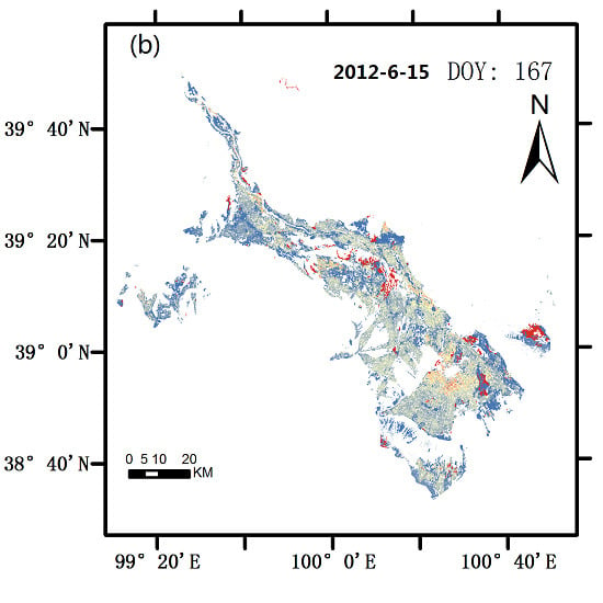
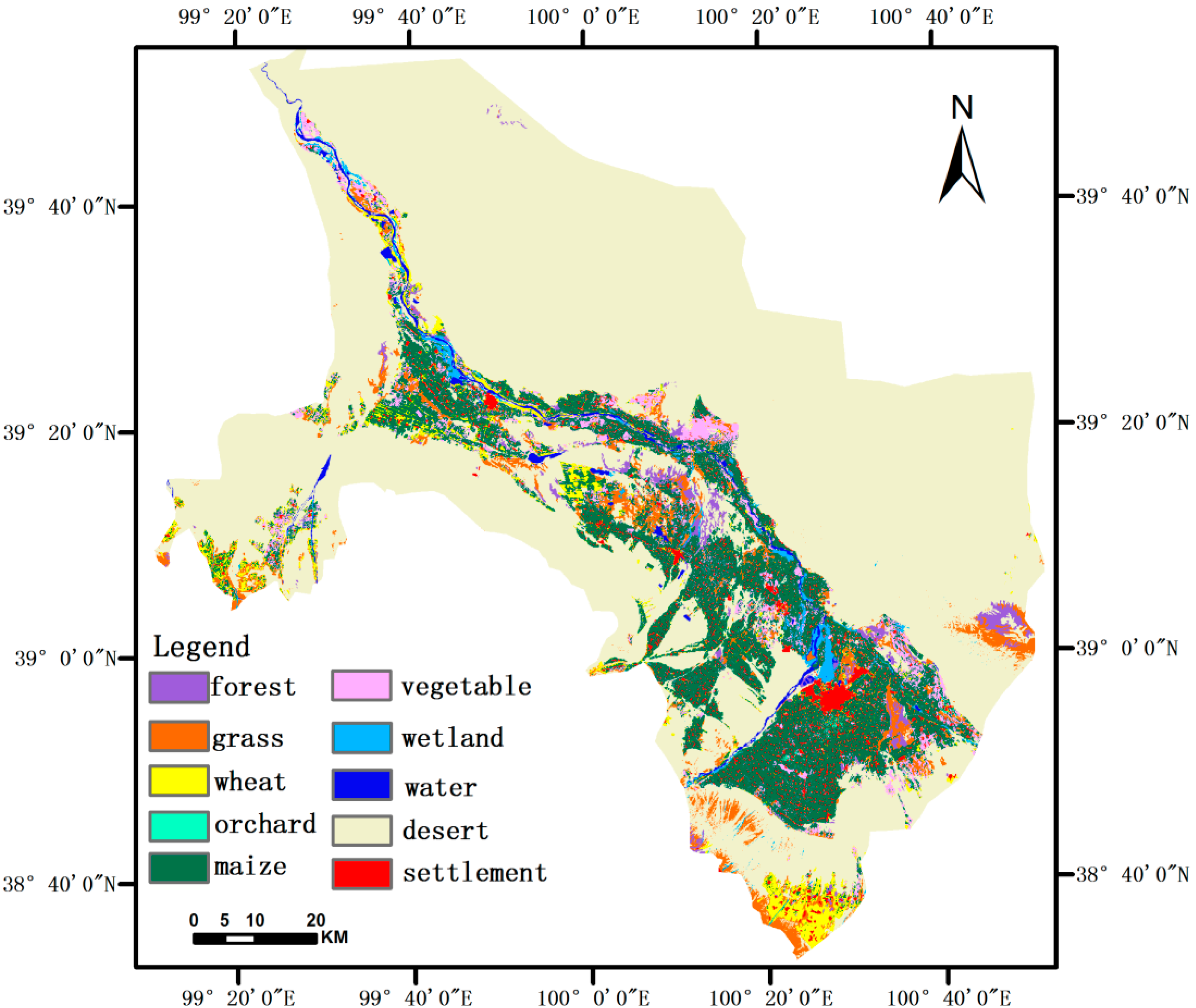
2.1. Study Area

The study area is located in the irrigated oasis in the middle reach of the Heihe River Basin around Zhangye, Gansu province, in the arid and semiarid region of northwest China. The Zhangye oasis is the main agricultural area in northwest China. Figure 1 is a 2012 land cover map of our study area. We produced this map by a supervised classification of multi-spectral data acquired by the HJ-1A/1B satellites. The training and evaluation samples were chosen from the available field survey data for the Zhangye oasis and high spatial resolution Google Earth images. The overall accuracy of the classification results reached 84.1%, and the Kappa coefficient was 0.81, which met the needs of this study.

The vegetation in the oasis is heavily dominated by crops (mainly spring corn, spring wheat, and vegetables, such as chili, celery, and cauliflower), with small areas of grasslands, wetlands (reed), and deciduous broad-leaved forests (Table 1). The oasis is surrounded by the Gobi desert (Figure 1) and has a continental dry climate [23]. The net radiation (Rn) can reach 800 w/m² during the growing season. Under sufficient irrigation, the latent heat flux (LE) in July and August can exceed 70% of the Rn on the oasis. During the non-growing season, the sensible heat flux (Hs) becomes dominant. In the last 30 years, several large field experiments have been carried out in this region, including the Atmosphere-Land Surface Processes Experiment conducted in the Heihe River Basin (HEIFI) [24] between 1988 and 1992, the Watershed Allied Telemetry Experimental Research (WATER) [25] experiment conducted between 2007 and 2009 and the Heihe Watershed Allied Telemetry Experimental Research (HiWATER) [26] study conducted between 2010 and 2015. The ground data we used are from the last of these experiments.

Figure 1. Land cover map of the middle reach of the Heihe River Basin in 2012.

Figure 1. Land cover map of the middle reach of the Heihe River Basin in 2012.

Table 1. The fractional abundances of the main vegetation classes over the study area resulting from the classification in Figure 1.

Vegetation Cover Class	Areal Percentage (%)	Area (km2)
Maize	53.6	1294
Wheat	12.7	276
Vegetables	14.5	350
Grassland	11.5	308
Forest	4.5	109
Orchard (apple tree)	0.2	5
Wetland	2.9	71

Table 1. The fractional abundances of the main vegetation classes over the study area resulting from the classification in Figure 1.

Vegetation Cover Class	Areal Percentage (%)	Area (km2)
Maize	53.6	1294
Wheat	12.7	276
Vegetables	14.5	350
Grassland	11.5	308
Forest	4.5	109
Orchard (apple tree)	0.2	5
Wetland	2.9	71

2.2. Data

2.2.1. In Situ Data

In this study, we collected growing season (May-September) EC data from field experiments at twelve sites. These relatively homogeneous sites included the main vegetation types in the middle reach of the Heihe River Basin, i.e., cropland, wetland, orchard, and forest vegetation, which represent a range of z_0m values from approximately 0.03 m to 0.8 m. All EC observations (10 maize sites, 1 orchard site, and 1 wetland site) are products of the Multi-Scale Observation Experiment on Evapotranspiration over heterogeneous land surfaces that was conducted in 2012 (MUSOEXE-2012) [27,28] within the framework of HiWATER. For each EC site, an eddy covariance (EC) system and an automatic meteorological station (AWS) were installed, with a minimum of one 3-dimensional sonic anemometer, one CO₂ and H₂O gas analyzer, one four-component radiometer, one rain gauge, one wind speed sensor and one wind vane. The various EC and radiometer devices of the different models produced by different manufacturers used in the MUSOEXE-2012 were inter-compared in the Baji Gobi desert west of Zhangye City (100°18′15.17″ E, 38°54′53.87″ N), and the inter-comparison campaign showed good agreement [27]. Table 2 contains the location information of all twelve EC sites.

Table 2. Information summary for the studied eddy covariance (EC) sites.

Site	Land Cover	Geographic Coordinates		Obs. Height	Period (2012)
EC01	Maize	100°21′54.83′′E	38°52′36.37′′N	3.8 m	29/5–18/9
EC02	Maize	100°21′14.63′′E	38°53′13.10′′N	3.7 m	7/6–19/9
EC03	Maize	100°21′2.34′′E	38°52′32.78′′N	3 m	3/6–18/9
EC04	Maize	100°21′35.00′′E	38°52′16.32′′N	4.6 m	28/5–21/9
EC05	Maize	100°22′35.28′′E	38°52′21.17′′N	3.2 m	28/5–21/9
EC06	Maize	100°23′44.53′′E	38°52′32.50′′N	4.8 m	4/6–17/9
EC07	Maize	100°20′31.12′′E	38°52′11.77′′N	3.5 m	29/5–18/9
EC08	Maize	100°21′58.79′′E	38°51′54.57′′N	3.5 m	28/5–21/9
EC09	Maize	100°21′11.23′′E	38°51′31.27′′N	4.6 m	30/5–21/9
EC10	Maize	100°22′20.09′′E	38°51′20.04′′N	4.5 m	25/5–15/9
EC11	Orchard	100°22′11.08′′E	38°50′42.43′′N	7 m	31/5–17/9
EC12	Wetland	100°26′47.04′′E	38°58′30.50′′N	5.2 m	25/6–26/9

Table 2. Information summary for the studied eddy covariance (EC) sites.

Site	Land Cover	Geographic Coordinates		Obs. Height	Period (2012)
EC01	Maize	100°21′54.83′′E	38°52′36.37′′N	3.8 m	29/5–18/9
EC02	Maize	100°21′14.63′′E	38°53′13.10′′N	3.7 m	7/6–19/9
EC03	Maize	100°21′2.34′′E	38°52′32.78′′N	3 m	3/6–18/9
EC04	Maize	100°21′35.00′′E	38°52′16.32′′N	4.6 m	28/5–21/9
EC05	Maize	100°22′35.28′′E	38°52′21.17′′N	3.2 m	28/5–21/9
EC06	Maize	100°23′44.53′′E	38°52′32.50′′N	4.8 m	4/6–17/9
EC07	Maize	100°20′31.12′′E	38°52′11.77′′N	3.5 m	29/5–18/9
EC08	Maize	100°21′58.79′′E	38°51′54.57′′N	3.5 m	28/5–21/9
EC09	Maize	100°21′11.23′′E	38°51′31.27′′N	4.6 m	30/5–21/9
EC10	Maize	100°22′20.09′′E	38°51′20.04′′N	4.5 m	25/5–15/9
EC11	Orchard	100°22′11.08′′E	38°50′42.43′′N	7 m	31/5–17/9
EC12	Wetland	100°26′47.04′′E	38°58′30.50′′N	5.2 m	25/6–26/9

The raw turbulence data were recorded at 10 Hz and averaged to 30 min intervals. Detailed information on data processing can be found in Liu et al. [28]. The following criteria were used for data selection: (1) u* > 0.15 m/s; (2) no rain; (3) −1 < (z−d)/L < 0.1.

The leaf area index (LAI) and vegetation height h were manually measured at each site listed in Table 2 and one vegetable site (100°21′29.26″E, 38°53′35.59″N) every few days during the growing season [29]. These measurements were used to estimate the empirical constants in Equations (7) and (8) (Section 3.2).

2.2.2. Remote Sensing Data

The HJ-1A/1B satellites were launched for environmental monitoring and disaster prevention by China on 6 September 2008 [30]. The data of the HJ-1A/1B satellites were obtained by combining the data acquired by the CCD (Charge Couple Device) sensors on both satellites (Table 3) resulting in a 2-day revisiting cycle with a 700 km swath from the visible to infrared wavelength spectrum.

Table 3. The main specifications of the HJ-1A/1B satellites and the Charge Couple Device (CCD) sensors.

Satellite Sensors	Band Number	Spectrum (mm)	Resolution (m)	Scene Width (km)	Revisiting Period (day)
HJ-1A/1B CCDs	1	0.43–0.52	30	360	4
	2	0.52–0.60
	3 (ρred)	0.63–0.69
	4 (ρnir)	0.76–0.90

Table 3. The main specifications of the HJ-1A/1B satellites and the Charge Couple Device (CCD) sensors.

Satellite Sensors	Band Number	Spectrum (mm)	Resolution (m)	Scene Width (km)	Revisiting Period (day)
HJ-1A/1B CCDs	1	0.43–0.52	30	360	4
	2	0.52–0.60
	3 (ρred)	0.63–0.69
	4 (ρnir)	0.76–0.90

3. Methodology

3.1. The R92 Remote Sensing Model to Estimate the Aerodynamic Roughness Length

We used the method proposed by Raupach (1992) [18] (R92 model). The foundation of the R92 model [18] is a precise analysis of the drag partition between the roughness elements and the underlying substrate. A turbulent wake is generated downwind of individual roughness elements, and, with increasing density, drag will increase before they begin to shelter each other, stabilize and eventually decrease again. The R92 model rests on two hypotheses: (1) shelter area and volume are related to the structure of the roughness elements and (2) the bulk shelter effects of the individual elements can be superimposed randomly. The ratio of aerodynamic roughness length to canopy height, z_0m/h, is expressed as follows:

$$z_{om}/h=(1-d/h)\exp (-k\frac{u_h}{u^{*}}-\eta )$$

(1)

where k is the von Kármán constant (taken as 0.41), z_0m (m) is aerodynamic roughness length, h (m) is the canopy height, u_h (m/s) is the mean horizontal wind velocity at h, u* (m/s) is friction velocity, d (m) is the zero-plane displacement height, and η is the profile influence function in R92, which accounts for the departure of the actual momentum diffusivity within the roughness sublayer from that above the roughness sublayer. In a study conducted by Raupach (1994), z_0m/h was insensitive to η. In this study, η = 0.193 was used as in R94.

In Equation (1), the ratio u_h/u* is related to the bulk drag coefficient (u*/u_h)², which was approximated by using the following dimensional analysis:

$$\frac{u^{*}}{u_h}=\frac{1}{\gamma }={(c_s+c_r\lambda )}^{1/2}/\exp (c\lambda \gamma /2) for \lambda <{\lambda }_{\max }$$

(2)

$$\frac{u^{*}}{u_h}={(\frac{u^{*}}{u_h})}_{\max } for \lambda >{\lambda }_{\max }$$

(3)

where c_s and c_r are the drag coefficients of the underlying substrate and an individual roughness element respectively, c is a constant accounting for overlapping effects of elements, and λ is the frontal area index, which is usually replaced by the canopy area index (Λ). For isotropically oriented canopy elements, λ and Λ are simply related as λ = Λ/2 [19]. Equation (3) implies that, the drag stress due to aerodynamic drag will remain constant when the areal density of roughness elements increases beyond a critical value.

In Equation (1), the ratio of the zero-plane displacement height to h, d/h, was deduced according to Thoms’s center-of-pressure hypothesis, which defines d as the vertical height of momentum absorption as [31]:

$$\frac{d}{h}=(\frac{\beta \mathrm{\Lambda }}{2+\beta \mathrm{\Lambda }})(1-\alpha {\gamma }^{-1}{\mathrm{\Lambda }}^{-1/2})$$

(4)

where α is an empirical constant associated with the geometric structure of roughness elements, and β is the ratio of c_r to c_s. The substrate drag coefficient, c_s, which is constant in agricultural areas, was assumed = 0.003, as proposed in R94.

In this method, five roughness parameters, c_r, α, c, (u*/u)_max and Λ_max, are crucial. Jasinski et al. [20] has applied the Method of Moments to estimate these five parameters for four IGBP land cover classes, evergreen needleleaf forests, grasslands, croplands, and open shrublands. In our study area, more vegetation types are found than the four Jasinski’s classes. Following the method of Borak et al. (2005) [21], all vegetation types in our study area are associated with most similar ones of the four classes parameterized by Jasinski et al. (2005) [20]. The parameters for each vegetation class in our study are shown in Table 4.

Table 4. Parameters applied in the R92 model for the study area of Heihe River Basin for 2012 (adapted from [20,21]).

Vegetation Cover Class	cr	(u*/u)max	c	α	Λmax
Forest	0.14	0.29	0.18	1.8	3.2
Orchard
Grass	0.23	0.32	0.28	1.53	2.3
Wetland
Maize	0.11	0.26	0.17	2.46	3.0
Wheat
Vegetables

Table 4. Parameters applied in the R92 model for the study area of Heihe River Basin for 2012 (adapted from [20,21]).

Vegetation Cover Class	cr	(u*/u)max	c	α	Λmax
Forest	0.14	0.29	0.18	1.8	3.2
Orchard
Grass	0.23	0.32	0.28	1.53	2.3
Wetland
Maize	0.11	0.26	0.17	2.46	3.0
Wheat
Vegetables

3.2. Canopy Structure Parameters

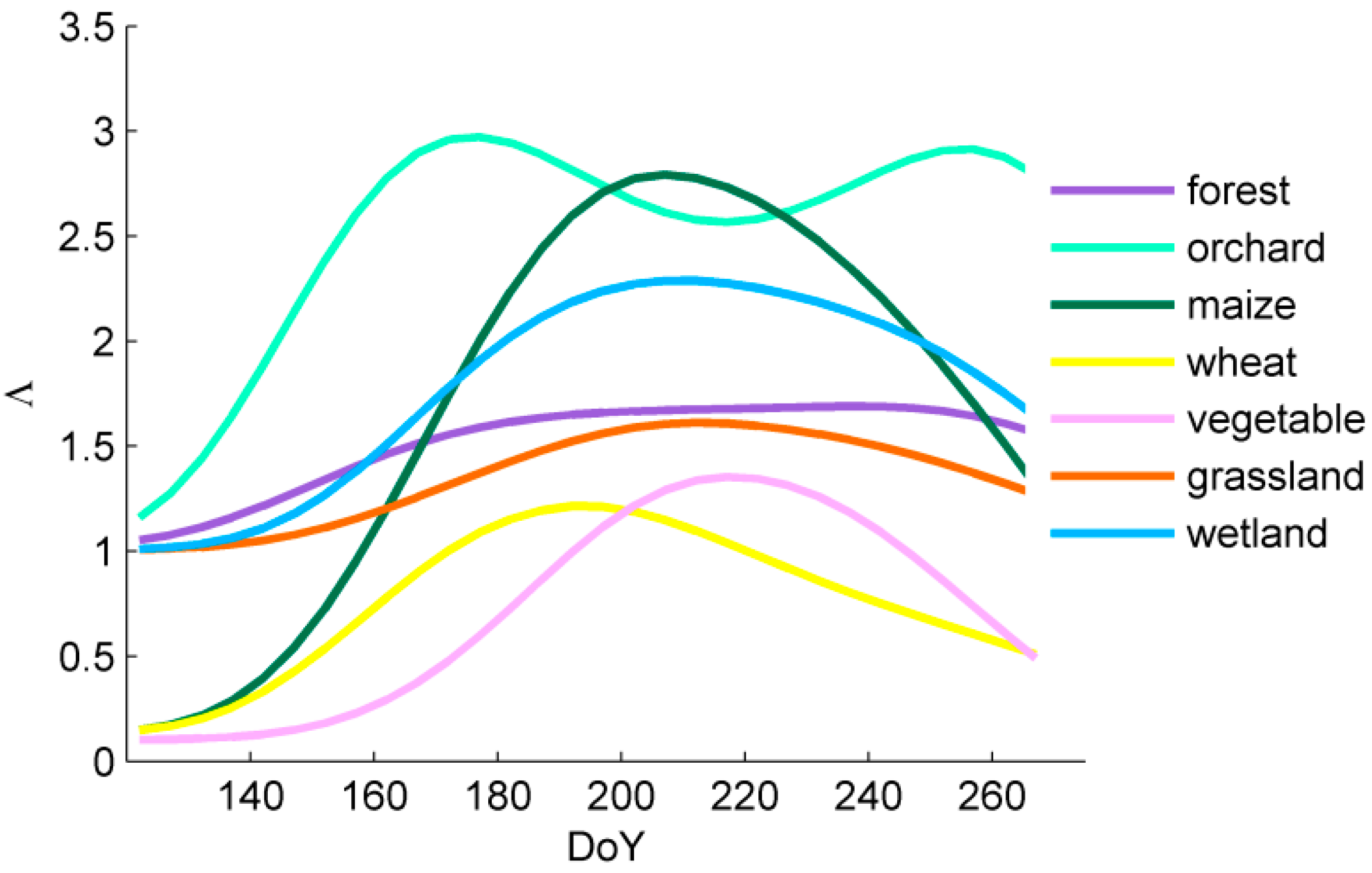
3.2.1. Canopy Area Index

The canopy area index Λ was used to express the canopy density, and composed of two parts: One-side area of all green canopy elements per unit ground area, i.e., the Leaf Area Index LAI, and the dead leaf and woody branches area, denoted as L_s:

$$\mathrm{\Lambda }=LAI+L_s$$

(5)

L_s was computed using the method of Zeng et al. (2002) [32] as follows:

$${L_s}^n=\max \left\{[\beta {L_s}^{n-1}+\max (LA{I}^{n-1}-LA{I}^n,0)],L_{s\min }\right\}$$

(6)

where L_smin is the minimum L_s, which consists of stems and dead leaves and depends on the vegetation type, n denotes the nth month, and the term (1−β) denotes the monthly removal rate of the dead leaves.

Satellite measurements of Red and NearInfraRed radiance can be used to determine the NDVI. Many studies, including early spectroradiometer measurements, documented a strong correlation between NDVI and ground measurements of LAI [33,34,35].

We used an empirical exponential relationship between NDVI and LAI to map LAI:

$$LAI(\mathrm{x},\mathrm{y},\mathrm{t})=a\times NDV{I}^b(\mathrm{x},\mathrm{y},\mathrm{t})$$

(7)

where a and b are empirical parameters that depend on vegetation type. Once the constants (a and b) for each vegetation type are known, LAI(x,y,t) can be mapped from NDVI(x,y,t), and the latter can be determined using the Red and NearInfraRed radiometric data acquired by the HJ-1A/1B satellites.

Field measurements of LAI during the growing season at the 12 EC sites and one vegetable site and the concurrent 30 m satellite NDVI were used to estimate the constants (a and b) for each vegetation type by applying Equation (7) and minimizing the least squares residuals. For wheat, grassland and forest where the field LAI measurements were not available, the empirical constants for Equation (7) were set to the same values as maize, reeds and orchard, respectively.

Finally, 5-day time series of LAI maps between May and September 2012 were produced. First, 37 cloud-free images (approximately 50% of the available 75 overpasses) of HJ-1A/1B with 30 m spatial resolution were pre-processed using an image-to-image geometric correction, followed by radiometric and atmosphere corrections; then, the 37 NDVI maps of 30 m spatial resolution were used to reconstruct a gap-free NDVI time series from May to September of 2012 using the Harmonic ANalysis of Time Series (HANTS) approach, and then the time series of LAI maps using Equation (7). The HANTS is a method for time series analysis and reconstruction based on the principles of Fourier Transform by decomposing a periodical series into Fourier components and it is a reliable method commonly used by many researchers for time series reconstruction [36]. HANTS has multiple advantages: It can deal with time series with irregularly spaced observations, detect outliers automatically, and capture the complex phenology of land cover by estimating the amplitude and phase of the periodic components used to model the NDVI time series [37,38]. Figure 2 shows an example of the original and reconstructed time series of NDVI using the HANTS approach.

Figure 2. Observations (dots) and the HANTS reconstructed (solid line) NDVI time series for one pixel in oasis area of Heihe River Basin in 2012.

Figure 2. Observations (dots) and the HANTS reconstructed (solid line) NDVI time series for one pixel in oasis area of Heihe River Basin in 2012.

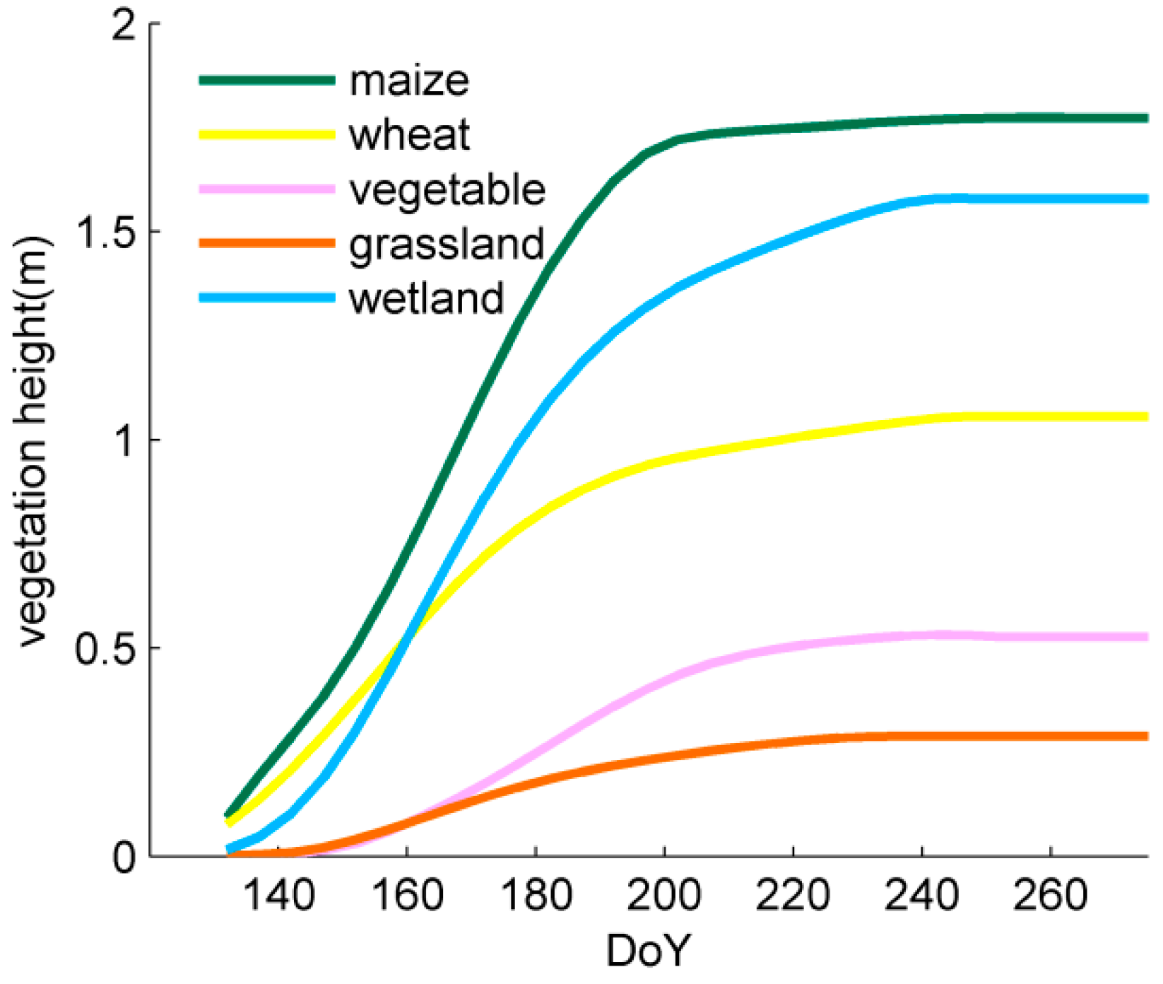
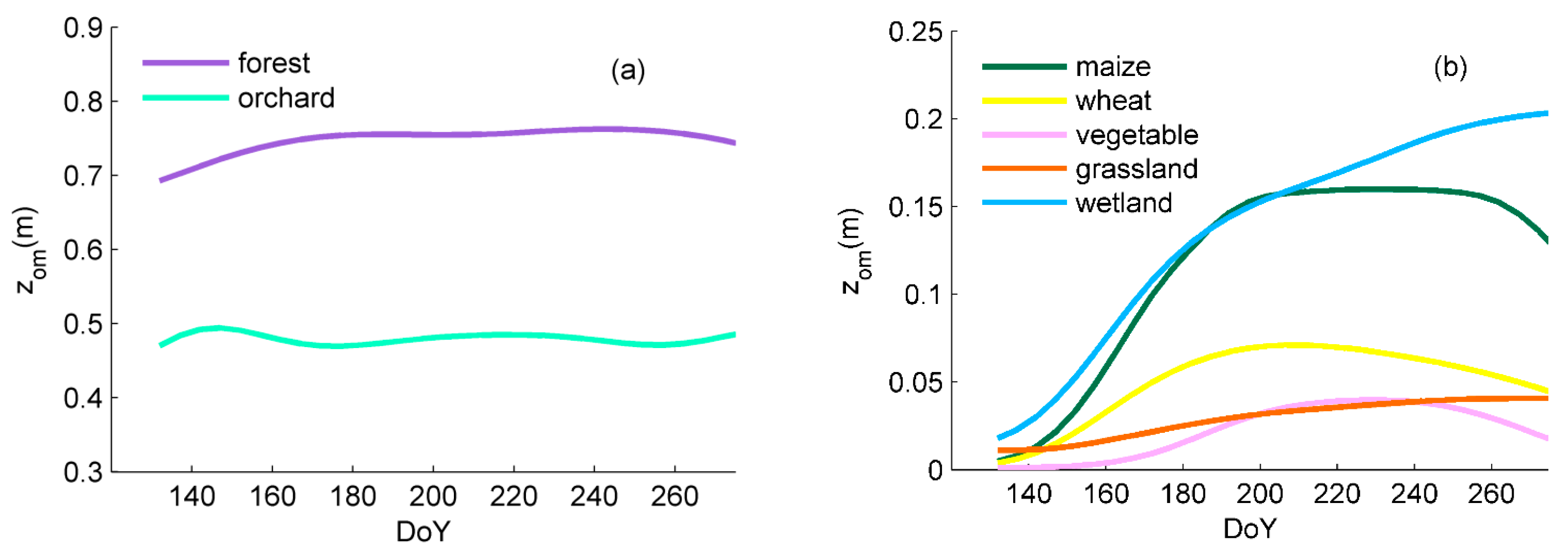
3.2.2. Vegetation Height

A map of vegetation canopy height is required to obtain a map of the aerodynamic roughness length parameter z_0m using the ratio z_0m/h estimated using Equation (1). Multi-spectral image data cannot be used to estimate directly canopy height. Satellite-based laser altimeters (i.e., the Geoscience Laser Altimeter System (GLAS) on Ice, Cloud, and land Elevation Satellite (ICEsat)-1/2 [39]) can provide measurements of vegetation height along the satellite ground-track, but the ICEsat across-track separation is about 60 km in the study area, so not sufficient for the purpose of this study. Airborne LiDAR with high spatial density detection could provide a higher resolution Digital Elevation Model (DEM) and Digital Surface Model (DSM) [40,41,42]. Vegetation height could be retrieved from the differences between the DSM and DEM values in the vegetated regions [7,9,10,11]. Airborne LiDAR data were acquired in the study area in 2012, and mapping h and z_0m by utilizing the LiDAR data will be the subject of another study in the near future.

We mapped vegetation height, h, using an empirical relationship with LAI, constructed using ground measurements collected at most of the sites listed above (Table 2). The evolution of h and LAI is nearly simultaneous in herbaceous crops like maize [43], in which case h/h_max = LAI/LAI_max at any time during the growing season, while in some species h tracks LAI and in other ones is the other way round. We used two empirical species-dependent parameters to account for this time-lag. The general form of our empirical relationship reads:

$$\frac{h}{h_{\max }}(\mathrm{x},\mathrm{y},\mathrm{t})=\min (\mathrm{e}\frac{LAI}{LA{I}_{\max }}(\mathrm{x},\mathrm{y},\mathrm{t})+f,1)$$

(8)

where e and f are the empirical species-dependent parameters: (1) e > 1 applies when the maximum vegetation height is reached earlier than the maximum LAI; (2) e < 1 when the maximum vegetation height is reached later than the maximum LAI; and (3) e = 1 and f = 0 in Equation (8) give h/h_max = LAI/LAI_max.

The detailed steps for vegetation height estimate are:

• Ground measurements of h and LAI for each annual herbaceous plant at the 11 EC sites (10 maize sites and 1 wetland site) and one vegetable site were divided by the highest observed value of h and LAI at each site.
• The normalized vegetation height (h/h_max) and leaf area index (LAI/LAI_max) values were used to estimate the constants (e, f) by applying Equation (8) and minimizing the least squares residuals for maize, wetland, and vegetable.
• For wheat and grasslands where no measurements of h and LAI were available, the empirical constants (e and f) in Equation (8) were set equal to those of maize and wetland vegetation, respectively.
• Equation (8), the values of the LAI_max and h_max and the revised empirical constants (e and f) were used to map vegetation height.

In Step 4, LAI_max was set to the maximum LAI (retrieved using Equation (7)) for each pixel over all dates, the h_max values for maize, wetland and vegetable were 1.8 m, 1.6 m and 0.5 m respectively, based on the field measurements, and the h_max values for wheat and grass were 1.0 m and 0.5 m, respectively, which is in agreement with past experiences. Furthermore, the vegetation heights of the orchard and forest were considered constant and were 5 m and 8 m, respectively, during the whole growing season based on local experience.

3.3. Local Roughness Lengths Estimated from Eddy-Covariance Measurements

The aerodynamic roughness length was estimated from the eddy covariance measurements at the sites listed in Table 2 to evaluate the map of aerodynamic roughness length constructed using Equation (1). In the boundary layer the Monin-Obukhov similarity theory applies and the scaled profile of the mean horizontal wind speed reads:

$$u(z)=\frac{u^{*}}{k}[\ln (\frac{z-d}{z_{om}})-{\psi }_m(\frac{z-d}{L})]$$

(9)

which can be expressed as:

$$\ln \frac{z-d}{z_{om}}=\frac{ku(z)}{u^{*}}+{\psi }_m(\frac{z-d}{L})$$

(10)

Here, L is the Monin-Obukhov length, ψ_m is the stability correction term and the displacement height d cannot be accurately derived from eddy covariance measurements. For dense and uniform vegetation the simple relationship d = 2/3 h applies [6] and was used in this study.

Chen and Wang (1993) found that the value of ku(z)/u* + ψ_m depends on stability, becoming higher under stable conditions and lower under unstable conditions. By plotting ku(z)/u* against (z − d)/L for both stable and unstable conditions, the two intercepts of the fitted lines, i.e., at ψ_m = 0 (neutral conditions), provide ln((z − d)/z_0m), which gives estimates z_0m values applying to the height of the EC measurements [44]. Our calculation of z_0m was done by applying this method. In this study, half hourly data were filtered based on criteria defined in Section 2.2.1. The filtered u(z), u* and L measurements for each 5 days period, during which we assumed that the aerodynamic roughness was constant, were divided into two groups: Stable and unstable conditions. Then, a robust regression method (MatLab @ routine “robustfit”), which can minimize the influences of outliers, was used to perform a linear fitting between (z − d)/L and ku(z)/u^* for stable and unstable data to obtain the intercepts. Finally, the degrees of freedom for unstable and stable data fittings were used as weighting factors to obtain the weighted intercept and the mean value of z_0m over 5 days. In addition, the standard error of the regression coefficient estimates was used to indicate the uncertainty of the observed z_0m.

4. Results

4.1. Canopy Structure Parameters Estimated from Remote Sensing Data

The coefficients (a and b) in Equation (7) for different vegetation types were obtained by least squares regression analysis using filed LAI measurements collected at the 12 EC sites and one vegetable site, and HJ-1A/1B NDVI data for the pixel of the corresponding site. The results together with the correlation coefficient (R) and the root mean square error (RMSE) are shown in Table 5. Due to lack of field LAI measurements over forest, wheat and grass, the relationships for these three surfaces were chosen to be same as those of orchard, maize, and wetland, respectively. A summary of the NDVI-LAI relationships is shown in Table 5.

Table 5. The empirical constants in the NDVI and LAI relations (Equation (7)) for different vegetation types used in this study.

Vegetation Type	(a, b)	R	RMSE	Number of Observations
Maize	(6.2784, 2.3011)	0.91	0.63	112
Wheat
Vegetable	(8.5609, 4.1193)	0.65	0.66	7
Orchard	(4.9578, 2.1994)	0.87	0.20	6
Forest
Wetland	(9.8268, 3.4428)	0.63	0.80	13
Grass

Table 5. The empirical constants in the NDVI and LAI relations (Equation (7)) for different vegetation types used in this study.

Vegetation Type	(a, b)	R	RMSE	Number of Observations
Maize	(6.2784, 2.3011)	0.91	0.63	112
Wheat
Vegetable	(8.5609, 4.1193)	0.65	0.66	7
Orchard	(4.9578, 2.1994)	0.87	0.20	6
Forest
Wetland	(9.8268, 3.4428)	0.63	0.80	13
Grass

The LAI map was constructed using Equation (7) applying the empirical coefficients in Table 5 to the HJ-1A/1B NDVI data in combination with the land cover map. For each 5 days period, the map of the canopy area index Λ was then produced by applying Equations (5) and (6) to the LAI map. Figure 3 depicts the evolution of the area-averaged Λ(t) for each vegetation class listed in Table 1. It is found the Λ(t) first began to increase during the vegetative growth stage and decrease during senescence. All vegetation types exhibit clear seasonal variations in Λ. Cropland and wetland vegetation showed a more pronounced seasonality because of the relatively low dead-leaf removal rate. Differences in the phases of Λ(t) among classes indicate differences in the phenology of vegetation.

Figure 3. Time series of the area-averaged canopy area index Λ(t) of different vegetation types during the growing season of 2012 in the middle reach of the Heihe River Basin.

Figure 3. Time series of the area-averaged canopy area index Λ(t) of different vegetation types during the growing season of 2012 in the middle reach of the Heihe River Basin.

The maps of vegetation height h(t) for annual herbaceous plants were constructed by applying Equation (8) to the LAI(t) maps. The empirical constants (e and f) in Equation (8) were obtained from the field canopy height and LAI measurements as explained above (see Section 3.2.2). Table 6 gives the resulting e and f values, together with the R and RMSE. A summary of the LAI-h results for annual herbaceous plants is shown in Table 6.

Table 6. The empirical parameters e and f in the h(LAI) relationship (Equation (8)) for different vegetation types.

Vegetable Type	(e, f)	R	RMSE
Maize	(0.95, −0.053)	0.96	0.085
Wheat
Vegetable	(0.83, 0.12)	0.98	0.042
Wetland	(0.58, 0.54)	1.0	0
Grassland

Table 6. The empirical parameters e and f in the h(LAI) relationship (Equation (8)) for different vegetation types.

Vegetable Type	(e, f)	R	RMSE
Maize	(0.95, −0.053)	0.96	0.085
Wheat
Vegetable	(0.83, 0.12)	0.98	0.042
Wetland	(0.58, 0.54)	1.0	0
Grassland

Figure 4. Time series of the area-averaged vegetation height of different herbaceous vegetation types during the growing season of 2012 in the middle reach of the Heihe River Basin.

Figure 4. Time series of the area-averaged vegetation height of different herbaceous vegetation types during the growing season of 2012 in the middle reach of the Heihe River Basin.

The maps of vegetation height h(t) for the whole study area were derived from the LAI(t) maps (estimated from HJ-1A/1B NDVI data) using the e and f values in Table 6 and the land cover map. The area-averaged vegetation height (Figure 4) of annual herbaceous plants increased over time as growing conditions became more favorable during the early growing season, and then stabilized in the mid growing season.

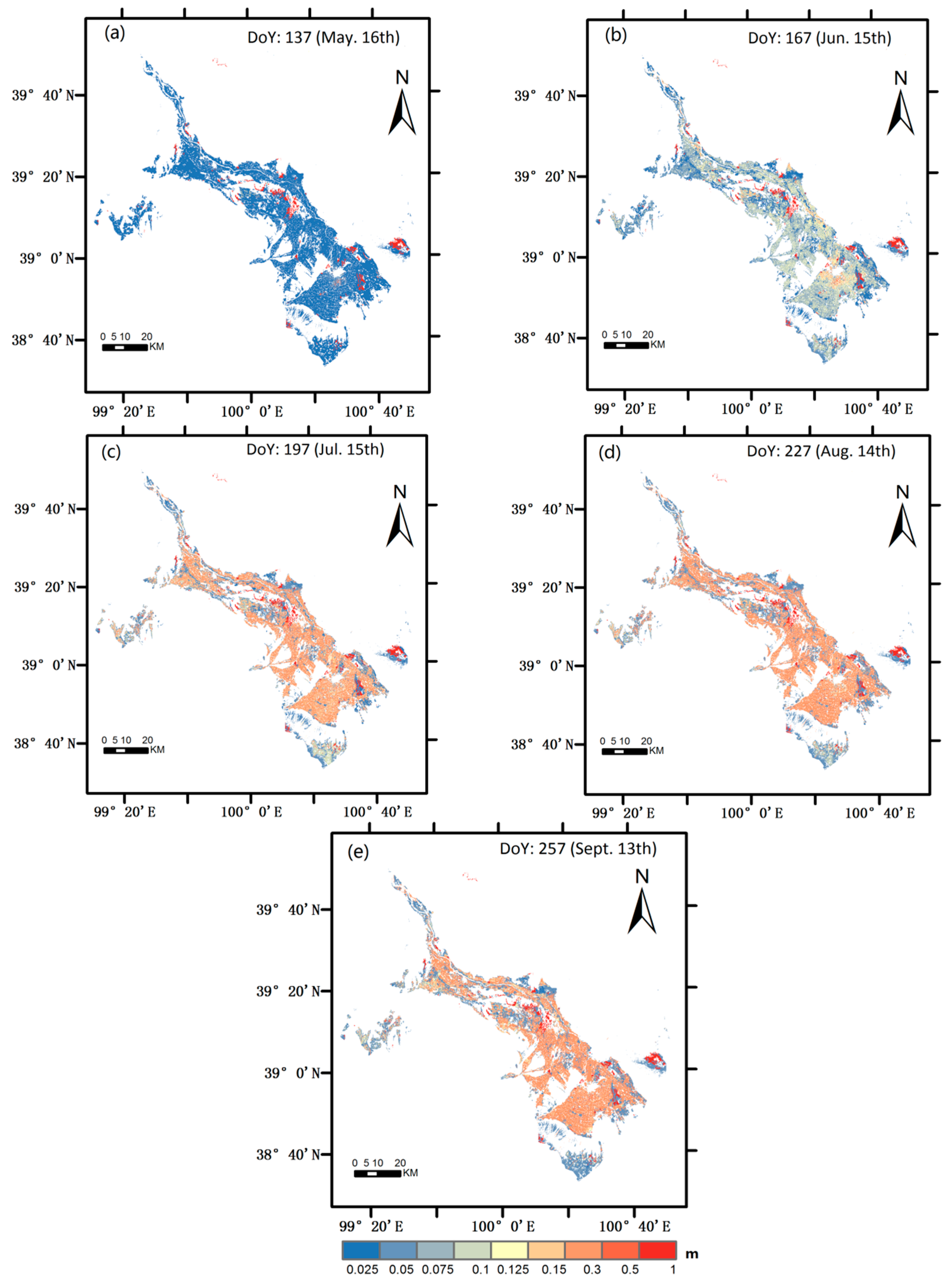
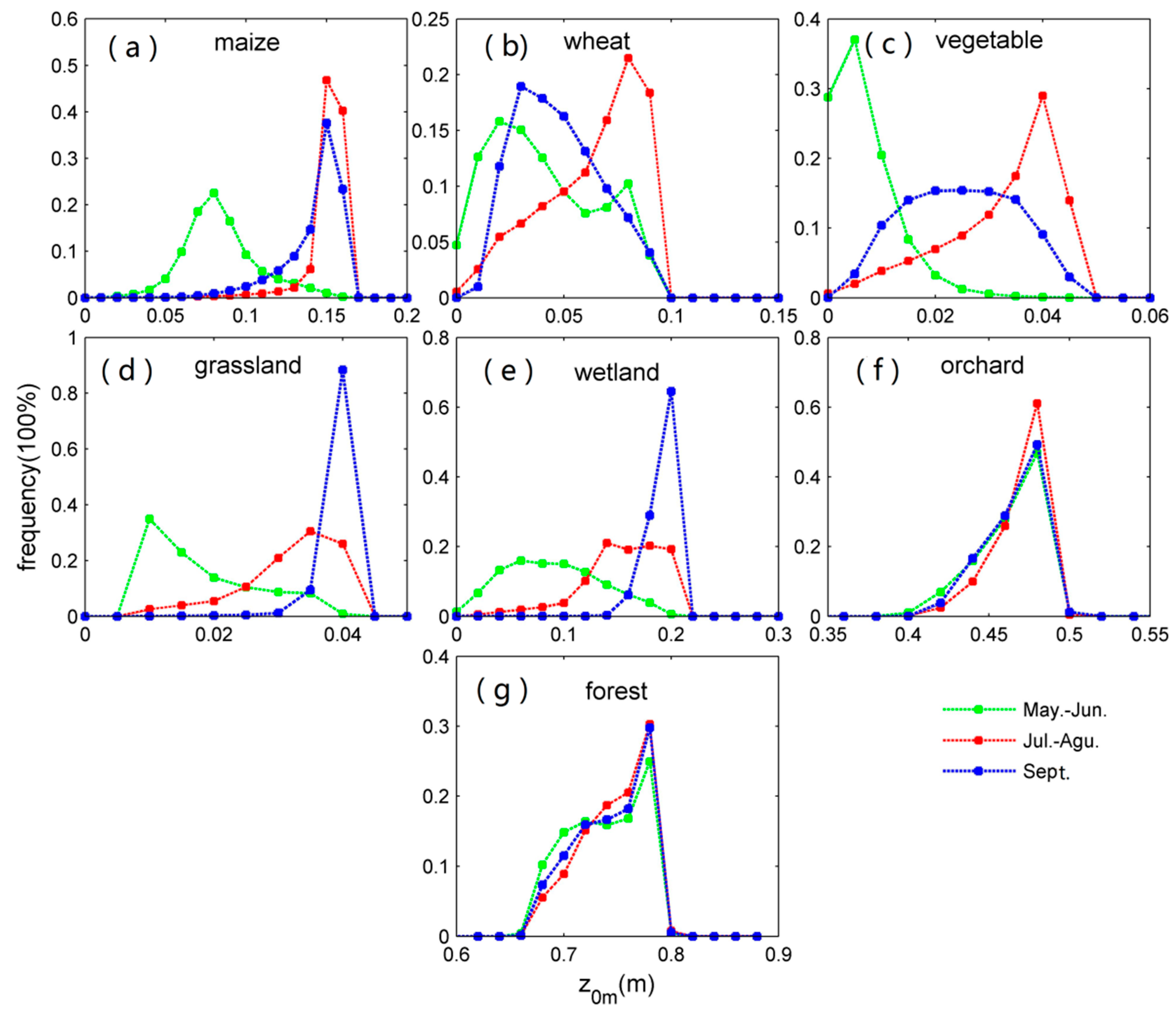
4.2. Regional Scale Aerodynamic Roughness Length

Maps of the aerodynamic roughness length z_0m(t) from May to September 2012 were constructed by applying Equation (1) using all canopy structure parameters derived from the HJ-1A/1B data and the model parameters described above. Figure 5 shows a time series of the area-averaged aerodynamic roughness length for different vegetation types from May to September of 2012. The magnitudes of the roughness length agree with values published for similar vegetation in the literature. Forest-type classes (orchard and forest) have much higher aerodynamic roughness lengths than non-forest type classes. The aerodynamic roughness lengths of the orchards and forests are about 0.46–0.5 m and 0.69–0.76 m (or approximately 0.09–0.1 h), respectively. The range of the aerodynamic roughness lengths for the non-forest vegetation types is larger (Figure 5b), and the roughness lengths of maize and wetland showed the largest variability. This result is consistent with the canopy area index Λ shown in Figure 3. The grasslands displayed smaller aerodynamic roughness lengths and narrower ranges than the agricultural classes because of the relatively low vegetation height, the smaller variability of the roughness elements density and the absence of harvesting. The aerodynamic roughness length of grasslands and wetlands did not begin to decrease until September 2012, which is consistent with a longer growing season and a late season leaf loss.

Figure 5. Time series of the regionally averaged aerodynamic roughness length during the growing season for different vegetation type: (a) forest vegetation; (b) non-forest vegetation.

Figure 5. Time series of the regionally averaged aerodynamic roughness length during the growing season for different vegetation type: (a) forest vegetation; (b) non-forest vegetation.

Figure 6 and Figure 7 illustrate the spatial distributions and histograms of the regional aerodynamic roughness length over the study area from May to September of 2012. To generate the histograms the roughness over the periods indicated (May–June, July–August and September, respectively) was averaged first. Next, the histogram over the entire region was calculated. The smallest spatial variability of the aerodynamic roughness lengths within class and among different classes occurred in May, when most crops were in the early stages of development. The greatest spatial differences among the different classes occurred in July and August, when most of the vegetable crops were in the booting stage. In Figure 6 and Figure 7, the spatial variability among the different classes is also apparent in September because the canopy area index Λ included the woody branches and dead leaves, which slows down the decrease in the density of the roughness elements and extends in time the apparent variability of the aerodynamic roughness length. The greatest variability occurred in June, mainly because the oasis is dominated by maize, and some deviations occurred in the sowing time. For the spring maize, June is the vegetative growth period and is characterized by the largest variability in vegetation height. In addition, the spatial variations of soil moisture, irrigation conditions, and soil fertility can contribute to the spatial variability in plant development, and the resulting spatial variability of the aerodynamic roughness length.

Figure 6. Aerodynamic roughness length in the period of May to September 2012 on days of year: (a) 137, (b) 167, (c) 197, (d) 227, and (e) 257.

Figure 6. Aerodynamic roughness length in the period of May to September 2012 on days of year: (a) 137, (b) 167, (c) 197, (d) 227, and (e) 257.

Figure 7. Histograms of z_0m in different growing seasons in 2012 (green curve: May–June; red curve: July–August; blue curve: September) for the different vegetation types over the study area (middle reach of Heihe River Basin): (a) maize; (b) wheat; (c) vegetable; (d) grassland; (e) wetland; (f) orchard and (g) forest.

Figure 7. Histograms of z_0m in different growing seasons in 2012 (green curve: May–June; red curve: July–August; blue curve: September) for the different vegetation types over the study area (middle reach of Heihe River Basin): (a) maize; (b) wheat; (c) vegetable; (d) grassland; (e) wetland; (f) orchard and (g) forest.

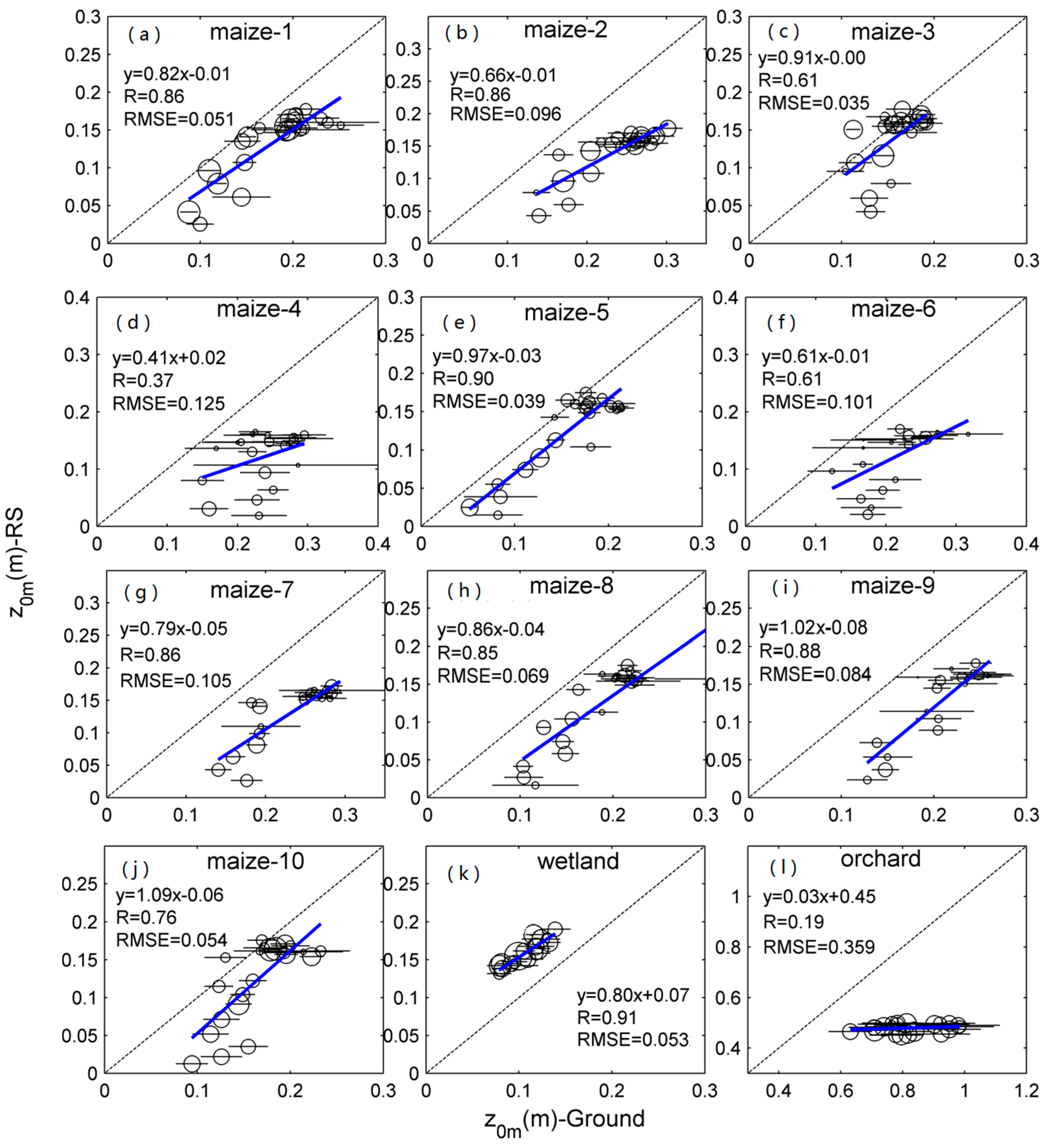
4.3. Validation and Comparison of the Aerodynamic Roughness Length Results

The aerodynamic roughness length estimated at the flux tower sites by the profile method (see Section 3.3) was used to validate the remote sensing model results for each site (see Figure 8). The error bars indicate the confidence intervals of the data, and the diameter of the circle in the middle of each error bar indicates the number of degrees of freedom for each robust regression (equivalent to the number of observations). Figure 8 shows that the greater the degrees of freedom the shorter are the error bars, which is to be expected. The coefficient of correlation, R and the RMSE are used to evaluate the results. Overall, the R92 method with the revised parameter sets of Jasinski et al. (2005) [20] provided seasonal trends and magnitudes that were similar to the EC derived aerodynamic roughness length, except for the orchard (Figure 8l). For the orchard (Figure 8l), the correlation between the remote sensing model estimates and the ground measured roughness length was rather poor. Compared with the other vegetation classes, the remote sensing (RS) results for the orchard class show less variability, this is partly due to the fact that the period of ground measurement in the orchard site was too short to capture the full growth of the fruit trees. In this case, longer time series of ground measurements should be added for further comparison. For wetlands, the model performs well, with relatively high R-values and low RMSE values. For maize, more sites are available for validation, and the RS roughness length model performed differently among different sites when compared with the measurements. Most of the sites showed high correlation, although the aerodynamic roughness length is usually underestimated by the remote sensing model.

Figure 8. Comparison between the estimated aerodynamic roughness length and the ground measurements from EC experimental sites (a–l) in the middle reach of the Heihe River Basin in 2012. Each circle is the area—Averaged value over five days. The diameters of the circle scale with the number of degrees of freedom (equivalent to the number of observations) for each robust regression. The error bars indicate the 95% confidence intervals of the regression estimate.

Figure 8. Comparison between the estimated aerodynamic roughness length and the ground measurements from EC experimental sites (a–l) in the middle reach of the Heihe River Basin in 2012. Each circle is the area—Averaged value over five days. The diameters of the circle scale with the number of degrees of freedom (equivalent to the number of observations) for each robust regression. The error bars indicate the 95% confidence intervals of the regression estimate.

5. Discussion

Although Jasinski et al. (2005) [20] used a broader range of canopy density and land cover types for parameters estimation, the parameters used in this model are still locally limited. The four vegetation types used by Jasinski et al. (2005) [20] may be insufficient to capture the geometric features of all vegetation types and finer model tuning may be needed (using ground measurements) for different vegetation classes.

Multi-spectral image data cannot replace local and direct measurements of aerodynamic roughness length. However, compared with ground measurements, remote sensing data have the advantages of wider coverage, relatively inexpensive and are easily obtained. Fine temporal and spatial resolution image data will be available as multiple satellites will provide similar measurements. This will make regional monitoring of aerodynamic roughness length easier, especially in heterogeneous areas. In this sense, deriving the land surface roughness length data using remote sensing observations is valuable.

The aerodynamic roughness length parameterizes momentum absorption, which can be affected by surrounding pixels, and the parameterization is non-linear. The aerodynamic roughness length is inherently related to the height over the surface of momentum flux measurements and their footprint. Different applications may require z_0m maps at different spatial resolutions. Strictly speaking, the aerodynamic roughness length is meaningful only over on homogeneous surfaces and within the surface layer in dynamic equilibrium with the underlying surface. Thus, the mixed pixels of coarse resolution multi-spectral image data will result in large error of estimate on both aerodynamic roughness length and turbulent fluxes. Thus, this study investigated the aerodynamic roughness length at fine spatial (30 m) and temporal (5 day) resolutions which is meaningful for regional scale modelers. Maps of aerodynamic roughness length at very high resolution are not really consistent with the physics underlying the logarithmic parameterization of u(z) and momentum flux. In addition, with the development of high resolution earth system models, which resolve increasingly finer scales of atmosphere dynamics, more knowledge of the relationships between the vegetation geometry and the model parameters relevant to a specific scale should be included [45].

As illustrated in Figure 8, deviations exist between EC estimations and model results, as well as among different vegetation classes. These deviations could occur for the following reasons: (1) Errors could exist in the EC measurements. Although the EC technique is usually the most accurate method for estimating aerodynamic roughness length, errors still exist when measurement conditions do not completely satisfy the basic assumptions, e.g., flat wind field, Taylor hypothesis, fast enough sampling rate, and enough averaging time for large scale eddies [46]. (2) The aerodynamic roughness itself is not only related to the geometry of the vegetation but also affected by meteorological conditions, such as the velocity and direction of the wind and the atmospheric stability. Different wind directions result in different measurement footprints i.e., deviations will appear in the aerodynamic roughness length when the land surface is heterogeneous. Figure 9a shows that the distribution of the z_0m values estimated from the EC measurements of maize (site 1) changes with wind direction. For site 1, three lines of windbreak trees south of the site result in a large value of z_0m for that wind direction (see Figure 9a). Furthermore, because vegetation is not a rigid body, its geometry can change with wind speed. Figure 9b implies that this effect occurs, where z_0m values decreased with increasing wind speed. Atmospheric stability provides an indication of thermal turbulence to some extent, and can also affect the EC measurements. (3) Topography may also result in a relatively large z_0m; however, this effect is negligible given the very flat topography of our study area.

Figure 9. Examples of aerodynamic roughness length changing with atmospheric conditions: (a) variation of EC-derived roughness with wind direction for maize site 1, indicating suboptimal fetch conditions in the south; (b) EC-derived roughness against wind speed for maize site 1, indicating the effect of crop bending with increased wind on the roughness length. The size of the circles in both (a) and (b) scales by the degrees of freedom in each fitting program, and error bars centered at each data point indicate 95% confidence intervals of the regression estimate.

Figure 9. Examples of aerodynamic roughness length changing with atmospheric conditions: (a) variation of EC-derived roughness with wind direction for maize site 1, indicating suboptimal fetch conditions in the south; (b) EC-derived roughness against wind speed for maize site 1, indicating the effect of crop bending with increased wind on the roughness length. The size of the circles in both (a) and (b) scales by the degrees of freedom in each fitting program, and error bars centered at each data point indicate 95% confidence intervals of the regression estimate.

6. Conclusions

The current research presents a practical approach for generating regional vegetation aerodynamic roughness lengths with fine temporal and spatial resolutions by combining remote sensing and ground measurements. In this study, the basic framework of the Raupach (1992) [18] (R92) model and the new parameters revised by Jasinsiki et al. (2005) [20] were adapted to derive the ratio of height-normalized aerodynamic roughness length to vegetation height, z_0m/h. The multi-spectral image data acquired by the HJ-1A/1B satellites were used to construct a land cover map based on a supervised classification method, fine resolution LAI maps and vegetation height maps using the empirical methods proposed in this paper, which performed well in our study area. Eventually, the aerodynamic roughness length, which is preferred by users, is generated rather than the ratio z_0m/h. The values and seasonal variations of aerodynamic roughness lengths for different vegetation types were different. Trees (orchard and forest) have much higher aerodynamic roughness lengths and less variability than the non-forest type classes.

Taking the advantage of the dense field EC tower measurements in the middle reach of the Heihe River Basin, the aerodynamic roughness length product was evaluated over different vegetation types. Aerodynamic roughness data from the EC tower sites were used as reference data and directly compared with the results derived from the remote sensing method using satellite data. Overall, the model performed well at wetland and maize sites but not at the orchard site. This discrepancy possibly occurred for several reasons, such as errors from EC ground measurements, and the accuracy of the model. The difference in the footprints between the ground measurements and remote sensing observations, combined with suboptimal fetch conditions from some of the former, may also explain some of this disagreement. Nevertheless, we are confident that implementing the R92 framework, enhanced by explicit vegetation height estimates, will provide improved distributed roughness length estimates for a range of applications.

References

1. Toda, M.; Sugita, M. Single level turbulence measurements to determine roughness parameters of complex terrain. J. Geophys. Res. 2003, 108. [Google Scholar] [CrossRef]
2. Brutsaert, W. Evaporation into the Atmosphere: Theory, History, and Applications; Springer: New York, NY, USA, 1982. [Google Scholar]
3. Stull, R.B. An Introduction to Boundary Layer Meteorology; Springer: New York, NY, USA, 1988; Volume 13. [Google Scholar]
4. Martano, P. Estimation of surface roughness length and displacement height from single-level sonic anemometer data. J. Appl. Meteorol. 2000, 39, 708–715. [Google Scholar] [CrossRef]
5. Garratt, J. The internal boundary layer—A review. Bound. Layer Meteorol. 1990, 50, 171–203. [Google Scholar] [CrossRef]
6. Maurer, K.D.; Hardiman, B.S.; Vogel, C.S.; Bohrer, G. Canopy-structure effects on surface roughness parameters: Observations in a Great Lakes mixed-deciduous forest. Agric. For. Meteorol. 2013, 177, 24–34. [Google Scholar] [CrossRef]
7. Colin, J.; Faivre, R. Aerodynamic roughness length estimation from very high-resolution imaging LiDAR observations over the Heihe basin in China. Hydrol. Earth Syst. Sci. 2010, 14, 2661–2669. [Google Scholar] [CrossRef]
8. Hasager, C.; Jensen, N. Surface-flux aggregation in heterogeneous terrain. Q. J. R. Meteorol. Soc. 1999, 125, 2075–2102. [Google Scholar] [CrossRef]
9. Menenti, M.; Ritchie, J.; Humes, K.; Parry, R.; Pachepsky, Y.; Gimenez, D.; Leguizamon, S. Estimation of aerodynamic roughness at various spatial scales. In Scaling up in Hydrology Using Remote Sensing; John Wiley and Sons: Chichester, UK, 1996; Volume 272. [Google Scholar]
10. Menenti, M.; Ritchie, J.C. Estimation of effective aerodynamic roughness of Walnut Gulch watershed with laser altimeter measurements. Water Resour. Res. 1994, 30, 1329–1337. [Google Scholar] [CrossRef]
11. De Vries, A.; Kustas, W.; Ritchie, J.; Klaassen, W.; Menenti, M.; Rango, A.; Prueger, J. Effective aerodynamic roughness estimated from airborne laser altimeter measurements of surface features. Int. J. Remote Sens. 2003, 24, 1545–1558. [Google Scholar] [CrossRef]
12. Sarwar, A.; Bill, R. Mapping evapotranspiration in the Indus Basin using ASTER data. Int. J. Remote Sens. 2007, 28, 5037–5046. [Google Scholar] [CrossRef]
13. Jia, L.; Wang, J.M.; Menenti, M. Estimation of area roughness length for momentum using remote sensing data and measurements in field. Sci. Atmos. Sin. 1999, 23, 632–640. [Google Scholar]
14. Lettau, H. Note on aerodynamic roughness-parameter estimation on the basis of roughness-element description. J. Appl. Meteorol. 1969, 8, 828–832. [Google Scholar] [CrossRef]
15. MacDonald, R.W.; Griffiths, R.F.; Hall, D.J. An improved method for the estimation of surface roughness of obstacle arrays. Atmos. Environ. 1998, 32, 1857–1864. [Google Scholar] [CrossRef]
16. Choudhury, B.; Monteith, J. A four-layer model for the heat budget of homogeneous land surfaces. Q. J. R. Meteorol. Soc. 1988, 114, 373–398. [Google Scholar] [CrossRef]
17. Shaw, R.H.; Pereira, A. Aerodynamic roughness of a plant canopy: A numerical experiment. Agric. Meteorol. 1982, 26, 51–65. [Google Scholar] [CrossRef]
18. Raupach, M.R. Drag and drag partition on rough surfaces. Bound. Layer Meteorol. 1992, 60, 375–395. [Google Scholar] [CrossRef]
19. Raupach, M. Simplified expressions for vegetation roughness length and zero-plane displacement as functions of canopy height and area index. Bound. Layer Meteorol. 1994, 71, 211–216. [Google Scholar] [CrossRef]
20. Jasinski, M.F.; Borak, J.; Crago, R. Bulk surface momentum parameters for satellite-derived vegetation fields. Agric. For. Meteorol. 2005, 133, 55–68. [Google Scholar] [CrossRef]
21. Borak, J.S.; Jasinski, M.F.; Crago, R.D. Time series vegetation aerodynamic roughness fields estimated from MODIS observations. Agric. For. Meteorol. 2005, 135, 252–268. [Google Scholar] [CrossRef]
22. Zhou, Y.; Ju, W.; Sun, X.; Wen, X.; Guan, D. Significant decrease of uncertainties in sensible heat flux simulation using temporally variable aerodynamic roughness in two typical forest ecosystems of China. J. Appl. Meteorol. Climatol. 2012, 51, 1099–1110. [Google Scholar] [CrossRef]
23. Zhang, J.-H.; Li, G.-D.; Nan, Z.-R.; Xiao, H.-L.; Zhao, Z.-S. The spatial distribution of soil organic carbon storage and change under different land uses in the middle of Heihe River. Sci. Geogr. Sin. 2011, 31, 982–988. [Google Scholar]
24. Wang, J.; Hu, Y.; Sahashi, K.; Mitsuta, Y. Outline of HEIFE field observations. In Proceedings of the International Symposium on Heife, Kyoto, Japan, 8–11 November 1993; pp. 22–29.
25. Li, X.; Li, X.; Li, Z.; Ma, M.; Wang, J.; Xiao, Q.; Liu, Q.; Che, T.; Chen, E.; Yan, G. Watershed allied telemetry experimental research. J. Geophys. Res. 2009, 114. [Google Scholar] [CrossRef]
26. Li, X.; Cheng, G.; Liu, S.; Xiao, Q.; Ma, M.; Jin, R.; Che, T.; Liu, Q.; Wang, W.; Qi, Y. Heihe watershed allied telemetry experimental research (HiWATER): Scientific objectives and experimental design. Bull. Am. Meteorol. Soc. 2013, 94, 1145–1160. [Google Scholar] [CrossRef]
27. Xu, Z.; Liu, S.; Li, X.; Shi, S.; Wang, J.; Zhu, Z.; Xu, T.; Wang, W.; Ma, M. Intercomparison of surface energy flux measurement systems used during the Hiwater-Musoexe. J. Geophys. Res. 2013, 118, 13140–113157. [Google Scholar]
28. Liu, S.; Xu, Z.; Wang, W.; Jia, Z.; Zhu, M.; Bai, J.; Wang, J. A comparison of eddy-covariance and large aperture scintillometer measurements with respect to the energy balance closure problem. Hydrol. Earth Syst. Sci. 2011, 15, 1291–1306. [Google Scholar] [CrossRef]
29. Hiwater Project Data. Available online: http://westdc.westgis.ac.cn (accessed on 20 November 2014).
30. HJ-1A/1B Satellite Data. Available online: http://218.247.138.121/DSSPlatform/index.html (accessed on 20 November 2014).
31. Thom, A. Momentum absorption by vegetation. Q. J. R. Meteorol. Soc. 1971, 97, 414–428. [Google Scholar] [CrossRef]
32. Zeng, X.B.; Shaikh, M.; Dai, Y.J.; Dickinson, R.E.; Myneni, R. Coupling of the common land model to the NCAR community climate model. J. Clim. 2002, 15, 1832–1854. [Google Scholar] [CrossRef]
33. Jordan, C.F. Derivation of leaf-area index from quality of light on the forest floor. Ecology 1969, 50, 663–666. [Google Scholar] [CrossRef]
34. Baret, F.; Guyot, G. Potentials and limits of vegetation indices for LAI and APAR assessment. Remote Sens. Environ. 1991, 35, 161–173. [Google Scholar] [CrossRef]
35. Chen, J.M.; Cihlar, J. Retrieving leaf area index of boreal conifer forests using Landsat TM images. Remote Sens. Environ. 1996, 55, 153–162. [Google Scholar] [CrossRef]
36. Verhoef, W.; Menenti, M.; Azzali, S. Cover a colour composite of NOAA-AVHRR-NDVI based on time series analysis (1981–1992). Int. J. Remote Sens. 1996, 17, 231–235. [Google Scholar] [CrossRef]
37. Menenti, M.; Azzali, S.; Verhoef, W.; van Swol, R. Mapping agroecological zones and time lag in vegetation growth by means of Fourier analysis of time series of NDVI images. Adv. Sp. Res. 1993, 13, 233–237. [Google Scholar] [CrossRef]
38. Jia, L.; Shang, H.; Hu, G.; Menenti, M. Phenological response of vegetation to upstream river flow in the Heihe River basin by time series analysis of MODIS data. Hydrol. Earth Syst. Sci. 2011, 15, 1047–1064. [Google Scholar] [CrossRef]
39. Harding, D.J.; Carabajal, C.C. ICESat waveform measurements of within-footprint topographic relief and vegetation vertical structure. Geophys. Res. Lett. 2005, 32. [Google Scholar] [CrossRef]
40. Flood, M. LiDAR activities and research priorities in the commercial sector. Int. Arch. Photogramm. Remote Sens. Spat. Inf. Sci. 2001, 34, 3–8. [Google Scholar]
41. Liu, X. Airborne LiDAR for DEM generation: Some critical issues. Prog. Phys. Geogr. 2008, 32, 31–49. [Google Scholar] [CrossRef]
42. Lim, K.; Treitz, P.; Wulder, M.; St-Onge, B.; Flood, M. LIDAR remote sensing of forest structure. Prog. Phys. Geogr. 2003, 27, 88–106. [Google Scholar] [CrossRef]
43. Gao, S.; Niu, Z.; Huang, N.; Hou, X. Estimating the Leaf Area Index, height and biomass of maize using HJ-1 and RADARSAT-2. Int. J. Appl. Earth Obs. Geoinf. 2013, 24, 1–8. [Google Scholar] [CrossRef]
44. Chen, J.Y.; Wang, J.M.; Mitsuaki, H. An independent method to determine the surface roughness length. Chin. J. Atmos. Sci. 1993, 17, 21–26. [Google Scholar]
45. Beven, K.J.; Cloke, H.L. Comment on “Hyperresolution global land surface modeling: Meeting a grand challenge for monitoring Earth’s terrestrial water” by Eric F. Wood et al. Water Resour. Res. 2012, 48. [Google Scholar] [CrossRef]
46. Aubinet, M.; Vesala, T.; Papale, D. Eddy Covariance: A Practical Guide to Measurement and Data Analysis; Springer: New York, NY, USA, 2012. [Google Scholar]