
Abstract
Carbon footprint is a key indicator of the contribution of food production to climate change and its importance is increasing worldwide. Although it has been used as a sustainability index for assessing production systems, it does not take into account many other biophysical environmental dimensions more relevant at the local scale, such as soil erosion, nutrient imbalance, and pesticide contamination. We estimated carbon footprint, fossil fuel energy use, soil erosion, nutrient imbalance, and risk of pesticide contamination for five real beef background-finishing systems with increasing levels of intensification in Uruguay, which were combinations of grazing rangelands (RL), seeded pastures (SP), and confined in feedlot (FL). Carbon footprint decreased from 16.7 (RL–RL) to 6.9 kg (SP–FL) CO2 eq kg body weight−1 (BW; 'eq': equivalent). Energy use was zero for RL–RL and increased up to 17.3 MJ kg BW−1 for SP–FL. Soil erosion values varied from 7.7 (RL–RL) to 14.8 kg of soil kg BW−1 (SP–FL). Nitrogen and phosphorus nutrient balances showed surpluses for systems with seeded pastures and feedlots while RL–RL was deficient. Pesticide contamination risk was zero for RL–RL, and increased up to 21.2 for SP–FL. For the range of systems studied with increasing use of inputs, trade-offs were observed between global and local environmental problems. These results demonstrate that several indicators are needed to evaluate the sustainability of livestock production systems.
Export citation and abstract BibTeX RIS

Content from this work may be used under the terms of the Creative Commons Attribution 3.0 licence. Any further distribution of this work must maintain attribution to the author(s) and the title of the work, journal citation and DOI.
1. Introduction
It is expected that by 2050 there will be 9 billion people on the planet. As a result, demand for food is growing rapidly, including meat which is predicted to grow 1.7% per year to 2030 and by 1.0% per year to 2050 (Food and Agriculture Organization (FAO) 2006). This increasing demand is associated with important structural changes in the livestock industry in many countries, such as intensification of production, vertical integration, geographic concentration, and up-scaling of production units (Steinfeld et al 2006). For instance, in Uruguay, Argentina, and southern Brazil beef cattle production systems were historically based on extensive grazing of natural rangelands and seeded pastures, but recently stocking rates have increased and confined systems (feedlots) have grown (Chiara and Ferreira 2012). At the same time, consumers and decision makers' awareness of the environmental impacts of food production has increased. Documented impacts of the livestock sector include: contributing to 18% of global greenhouse gas emissions (GHG), consuming 8% of global drinkable water, polluting water through animal wastes, fertilizers and pesticides, reducing biodiversity and degrading lands (Steinfeld et al 2006).
The livestock industry contributes to GHG emissions mainly through enteric methane emissions from rumen digestion, nitrous oxide (N2O) from manure and fertilizers, and carbon dioxide (CO2) from production for crops for feed. Crop production for livestock feed also impacts on the environment through soil erosion, pesticides, fertilizers and the consumption of fossil fuel energy, a non-renewable resource. Pesticides impact on water, soil, non-target organisms and on humans, while the use of fertilizers also increases the rate of supply of nutrients and organic substances to water bodies, accelerating eutrophication processes.
The carbon footprint is an indicator of GHG emissions associated with products and services, with growing international importance. Calculating GHG emissions helps to account for a global environmental problem but can mislead the evaluation of sustainability of livestock systems to an oversimplified view, because it does not account for other environmental impacts of local relevance. Furthermore, international reports analyzing beef systems sustainability (Capper 2012, Beauchemin et al 2010, Pelletier et al 2010, Ogino et al 2004, Subak 1999) do not account for typical production systems of temperate south-America, where 22% of the exported beef in the world comes from FAOSTAT (2012). Therefore the aim of this study was to estimate the carbon footprint, fossil energy consumption, soil erosion, nutrient balance, and pesticide contamination risk of beef-finishing production systems of Uruguay with different levels of intensification.
2. Materials and methods
We calculated GHG emissions, erosion rates, energy consumption, nutrient (phosphorus and nitrogen) balance, and pesticide contamination risk for five combinations of background-finishing beef systems from the eastern department of Rocha, Uruguay using a set of available models. These systems represent a gradient of situations with different intensification level, achieving different productivities as a result of technological advances and higher input use both through fertilizers and mechanization.
We defined our system's boundaries from the animals entering the finishing system to the gate, going to slaughter. We did not take into account cow–calf systems since they are homogeneous around the country and the most important differences arise at the final stage.
2.1. Production systems description
In the region assumed for this study (department of Rocha), beef production accounts for 60% of farmers' income and 82% of agricultural land use (MGAP 2002) with an average stocking rate of 0.67 animal units (AU) ha−1.1 This area was selected because it is representative of Uruguay where beef production accounts for 50% of the farmers, 77% of land use (MGAP 2002) and has an average stocking rate of 0.68 AU ha−1.
The dominant landscape in the area combines hills and slight slopes (3–5%) with valleys with flooding periods during winter. In short distances (1 km) a high diversity of soils can be found, from shallow soils (20–30 cm) in the upper part of hills, to deep (80 cm−1 m) and fertile (6% of soil organic matter) (MGAP 1976). Annual mean precipitation in the region is 1015 mm, with a homogeneous monthly distribution.
Based on previous published literature and expert opinion, we identified two background and three finishing beef production stages (Ferrés 2004, Berretta 2003). The background stage comprises the growth period between 150 and 350 kg; all these systems were based on grazing, either natural rangelands (RL) or seeded pastures (SP) (Berretta 2003, Berretta et al 2000, Risso 1997). Finishing is the stage between 350 and the slaughter weight of 500 kg and is based on RL, SP and feedlot (FL) (Ferrés 2004, Chiara and Ferreira 2012, Berretta 2003, Berretta et al 2000, Risso 1997). The most common systems in the region are five different combinations of these background-finishing stages: RL–RL, RL–SP, SP–SP, RL–FL and SP–FL. We then identified five representative commercial farmers in the region, who kept good records of their management and production through interviews with local extension agents. Through interviews we collected the necessary information to describe the detailed diets, weight gains and land use allocation for one typical cycle of production. The nutritional requirements of each animal were determined using average weight gain, following National Research Council (NRC) (1996) and Agricultural and Forage Research Council (AFRC) (1993) guidelines for British breed steers. Feed intake was assumed as 100% of supplements (grain or hay) offered or forage utilized, assuming 70% of utilization for forage estimated yield for seeded pastures and 60% for rangelands (Holechek et al 1989). Average daily gain was assumed constant for the entire period for each system. Inputs for nutritional calculations were initial and final animal weight, average daily gain, and feed characteristics (type of diet and how it was offered). With this information, nutritional requirements were calculated, as well as the amount of forage and grain required to fulfil those requirements, based on nutritional characteristics of forages and concentrates reported by Mieres et al (2004).
Each system nutritional characteristics and required time to finish the steers are presented in table 1. Crop–pasture rotations in SP systems consisted of two years of crops and three years of pastures. The crops for SP (background) were ryegrass (Lolium multiflorum Lam.) and sorghum (Sorghum bicolor (L.) Moench), and for SP (finishing) the crops were sorghum (Sorghum bicolor (L.) Moench) and rice (Oryza sativa). All seeded pastures were a mixture of fescue (Festuca arundinacea Schreb.) + white clover (Trifolium repens L.) and birds foot trefoil (Lotus corniculatus L.) For feedlot systems continuous cropping of rice and sorghum (Sorghum bicolor (L.) Moench) were considered. All rotations managed soil under no-tillage.
Table 1. Diet characteristics, average daily gain, and time to finish steers of two background and three finishing beef systems of eastern Uruguay. (Note: BW: body weight.)
| System | Background (150–350 kg BW) | Finishing (350–500 kg BW) | |||
|---|---|---|---|---|---|
| Rangeland | Seeded pasture | Rangeland | Seeded pasture | Feedlot | |
| Diet compositionb (Dry matter %) | 100% Native pasture | Seeded pasture (61%), native pasture (30%) and sorghum grain (9%) | 100% Native pasture | Seeded pasture (93%), sorghum grain (6.5%), rice bran (0.5%) | Sorghum grain (60.5%), rice bran (12%), rice husk (14%), rice hay (8.5%), vitamins and minerals (5%) |
| Dry matter digestibility (%)a | 55 | 66 | 55 | 68.5 | 83.5 |
| Crude protein in diet (%)a | 9.5 | 15 | 9.5 | 14.5 | 9.7 |
| Metabolizable energy in diet (Mcal animal d−1)a | 15.9 | 19.2 | 19 | 20.5 | 40.8 |
| Average daily gain (kg animal d−1)b | 0.4 | 0.7 | 0.4 | 0.7 | 1.4 |
| Dry matter intake (kg/animal/day)a | 9.9 | 7.9 | 12 | 8.4 | 13.2 |
| Time to achieve final weight (days)b,c | 486 | 285 | 366 | 214 | 102 |
aCalculated from coefficients from Mieres et al (2004). bInformation provided by farmers. cTime to go from 150 to 350 kg in background and from 350 to 500 in finishing systems.
Nutritional requirements were used to calculate the relative area for each system needed to produce the required amount of feed, using national technical coefficients for crop and forage production (table 2). These outputs were the activity data inputs for calculating environmental impacts.
Table 2. Yield and nutritional content of feedstuffs considered.
| Rangelandc | Seeded pastured | Sorghum grain | Rice bran | Rice husk | |
|---|---|---|---|---|---|
| Yield (Mg of DM ha−1)a | 5.5 | 7.5 | 4.1 | 1.5e | 0.7e |
| Organic matter digestibility (%)b | 55 | 67 | 85 | 44 | 73 |
| Crude protein (%)b | 10 | 15 | 8.6 | 10 | 15 |
| Metabolizable energy (Mcal/kg DM)b | 2.1 | 2.4 | 3.3 | 2.2 | 2.2 |
aSource: rangeland: Leborgne (1983), seeded pasture: Díaz (1995) and crops: MGAP (2011a). bMieres et al (2004). cRangeland from Fray Bentos Unit (Leborgne 1983). dAverage values per year in a 3-year pasture. eActual grain yield is 7.6 Mg ha−1 but only 20% of the harvested grain goes to bran and 10% to husk.
Farmers and farm managers provided the inputs used in one cycle to produce the forages and grains on each system (table 3).
Table 3. Inputs and estimated area to produce the feed consumed by animals in two background and three finishing beef systems of eastern Uruguay.
| Rangeland | Seeded pasture | Feedlot | |
|---|---|---|---|
| N fertilizer (kg N ha−1) | 0 | 9 | 67 |
| Diesel (L ha−1) | 0 | 12 | 30 |
| Glyphosate (kg ha−1)a | 0.0 | 3.3 | 7.4 |
| 2,4 D amina (kg ha−1)a | 0.0 | 1.5 | 0.04 |
| Atrazine (kg ha−1)a | 0.0 | 0.2 | 1.6 |
| Clomazone (kg ha−1) | 0.0 | 0.001 | 0.1 |
| Propanil (kg ha−1)a | 0.0 | 0.007 | 0.01 |
| Quinclorac (kg ha−1)a | 0.0 | 0.002 | 1.5 |
| Pesticides (kg ha−1)a,b | 0.0 | 5.0 | 10.7 |
| Area of the system (ha animal−1)c | 0.9 | 0.7 | 0.4 |
aActive ingredient. bTotal pesticide use. cTotal area of the rotation needed to feed one animal.
2.2. Greenhouse gas emissions
Methane (CH4), nitrous oxide (N2O) and carbon dioxide (CO2) were considered in calculating GHG emissions based on Intergovernmental Panel on Climate Change (IPCC) equations (IPCC 2006). The equations for enteric fermentation, manure management (CH4), production and distribution of animal's feed (N2O and CO2) are presented in table S1 (available at stacks.iop.org/ERL/8/035052/mmedia) and coefficients and emission factors in table 4. Methane emissions from enteric fermentation were estimated based on the energy density (gross energy consumed per day) and the quality of the diet (digestibility and crude protein). Greenhouse gas emissions from manure management are affected by both the animal's nutrition and the effluent treatment system. Nitrous oxide emissions from the production of feed sources include direct and indirect GHG emissions from both the manure and the urine deposited on pasture in grazing systems and from the manure management system in feedlots. Carbon dioxide emissions include fossil fuel combustion machinery used in farming and food distribution.
Table 4. Coefficients and emission factors to calculate GHG emissions of two background and three finishing beef systems of eastern Uruguay. (Note: Ym: conversion methane factor (% of gross energy lost as methane); GE: gross energy intake (MJ d−1); Bo: maximum methane producing capacity for manure produced by livestock category (m3 CH4 kg of VS/excreted); VS: excreted volatile solids (kg MS animal d−1); MCF: methane conversion factors for manure management system in the climate region; EF3: emission factor according to the manure management and region; EF4: emission factor according to manure management system; EF5: emission factor according to manure management system; EFc: fuel factor emission (gas oil) (2.98 kg CO2 eq kg fuel−1).)
| Coefficient/ emission factor | Source | |
|---|---|---|
| CH4 | ||
| Ym (Feedlot) (% GE) | 3 | IPCC (2006), table 10.3 |
| Ym (Grazing) (% GE) | 6.5 | |
| Bo (m3 CH4 kg of VS−1) | 0.1 | IPCC (2006), table 10A-5 |
| MCF (Feedlot) | 32 | IPCC (2006), table 10A-5 |
| MCF (Grazing) | 1.5 | |
| N2O | ||
| EF3 (kg N2O–N) | 0.02 | IPCC (2006), table 11.1 |
| EF4 (kg N2O–N) | 0.01 | IPCC (2006), table 11.3 |
| EF5 (kg N2O–N) | 0.0075 | IPCC (2006), tables 10.5 and 11.3 |
| CO2 | ||
| EFc (kg CO2 eq kg gas oil−1) | 2.9 | IPCC (2006) and MIEM (2010) |
| Inputs emission factors | ||
| Herbicides (CO2 eq L−1)a | 18.3 | Spielmann et al (2007), Ledgard (2011), MGAP (2011b) and Carámbula (1981) |
| Insecticides (CO2 eq L−1)a | 14.8 | |
| Seeds (kg CO2 kg−1)a | 0.2 | |
| Fertilizers (kg CO2 kg−1)a | 0.4 | |
Extraction, manufacture and transport of inputs, direct and indirect GHG emissions from N fertilization (N2O), and diesel combustion (CO2) for feed production were included in calculations. Feedlot systems use diesel combustion for feed distribution.
A tier 2 IPCC (2006) approach and information from Ministerio de Industria, Energía y Minería (MIEM) (2010) were used in calculating diesel and glyphosate emission factors. Methodology described by Spielmann et al (2007) and 9.0 × 10⁻³ kg CO2-eq Mg km−1 from (Ledgard 2011) was used to calculate emission factors of extraction of raw materials, manufacture, and transport of fertilizers and pesticides. Means of transportation and amounts imported in the last 5 years were obtained from MGAP (2011b). Greenhouse gas emissions derived from seed production were calculated by the simulation of one production cycle and a seed harvesting index from Carámbula (1981).
Carbon stock in soil was assumed to remain constant, as recommended by IPCC (2006). Global warming potential was 1 for CO2, 25 for CH4 and 298 for N2O for 100 years (Forster et al 2007). Greenhouse gas emissions were expressed in kg of CO2 equivalent per kg of body weight gained by the animals in the background and finishing period (BW) and by carcass weight (CW) considering a slaughter yield of 58.3% (steer's average for year 2011) (INAC 2012).
2.3. Energy use
Fossil fuel energy consumption was estimated using the coefficients in table 5 and farm-specific data from tables 2, 3 and 12 (yields, inputs and total area per animal). The energy use per kg of live weight gained was estimated over one growing cycle and expressed in MJ kg body weight−1 (BW).
Table 5. Coefficients to calculate energy consumption of two background and three finishing beef systems of eastern Uruguay.
| Input | References | |
|---|---|---|
| Gas oil (MJ l−1) | 39 | Llanos (2011) |
| Cropping activities (MJ ha−1)a | 223 | Llanos (2011) |
| Pesticides (MJ kg−1)a | 280 | West and Marland (2002) |
| Fertilizers (MJ kg−1)a | 33 | Kongshaug (1998) |
| Seeds (MJ kg−1)a | 37 | Llanos (2011) |
2.4. Soil erosion
Soil erosion rates for each system were estimated using EROSION 5.0 (García Préchac et al 2005), a model based on the Universal Soil Loss Equation (Renard et al 1994) and its later Revision (USLE/RUSLE) adapted and calibrated for Uruguay soils.
The USLE is a multiplication of factors, derived from climate (erosivity), topography (erodability, length and inclination of slope) and management (use and management and mechanical activity).
Rain erosivity factor is the rainfall energy applied to soil, derived from local meteorological data (J ha−1). Soil erodability is the average soil lost by unit of erosivity on bare soil (Mg J−1). Length slope factor is the relation between erosion at a given length and the one occurring at 22.1 m, when all other factors remain constant. The slope inclination factor is the relation between erosion at a given slope and the one occurring at 9% slope, when all other factors remain constant. The use and management factor is the relation between soil erosion under a set system and the erosion that would occur from a soil under bare soil, when all other factors remain constant. The mechanical activity factor is the relation between soil erosion under a determined mechanical activity and that occurring under a standard tillage in favor of the slope, when all other factors remain constant.
The same location (department of Rocha, SE of Uruguay) was considered for all systems, as well as soil type (Brunosol subeutrico típico—Typic Argiudolls) (MGAP 1976) and topography with slopes of 3% and 100 m long. These erosion rates (in kg ha−1) were multiplied by the area needed to produce feed to finish one animal to calculate total erosion (in kg), and expressed as kg of soil loss per kg of animal BW.
2.5. Nutrient balance
Nitrogen (N) and phosphorus (P) nutrient imbalance ratio (NIR) was calculated for each system using the methodology proposed by Koelsch and Lesoing (1999). This indicator is a ratio between nutrient outputs and inputs used in the system. Values over one represent nutrient surpluses (higher surpluses represent higher risks of water contamination) and values under one represent that nutrients are being exported at a higher rate than incorporated in the system.
Nitrogen inputs considered fertilizers and nitrogen biological fixation from legume pastures while the body weight gained in the period was considered as output. On rangelands nitrogen biological fixation is not accounted since the presence of legumes in the botanical composition of this communities are relatively low (Nabinger et al 2000). Phosphorus inputs considered fertilizers as inputs and the body weight gained in the period as output.
Coefficients for these calculations are presented in table 6.
Table 6. Coefficients and equations used in nutrient (N and P) imbalance calculations. (Note: NBF: nitrogen biological fixation; EBW: empty body weight (55% of the animal's live weight, assuming British breed steers).)
| Coefficient | Value/equation | Reference |
|---|---|---|
| Animal's N content |
|
NRC (1996) |
| % N NBF of Legume pasture (25–90%) 1∘ year of production | 18% of harvested weight | Koelsch and Lesoing (1999) |
| % N NBF of Legume pasture (25–90%) 2∘ year of production | 36% of harvested weight | |
| % N NBF of Soybeans | 40% of harvested weight | |
| Animals P content | 0.69% of EBW | NRC (1996) |
2.6. Pesticide contamination risk
We based our calculations on an index proposed by Viglizzo et al (2006), which considers each pesticide toxicity values (LD-50), solubility (Ksp), adsorption (Koc) and the time required for the pesticide to decline to 50% under field conditions. These values were obtained from the pesticide properties database (PPDB) (2009). Products used on each system and its coefficients are presented in table 7.
Table 7. Solubility (Ksp), adsorption (Koc), time for 50% decomposition (T1/2) and lethal dose-50 (LD-50) for pesticides used in two background and three beef-finishing systems of eastern Uruguay. Values used to calculate the pesticide contamination risk (PPDB 2009).
| Active ingredient | Ksp (g g−1) | Koc (g g−1) | T1/2 (days) | 1000/LD50 (mg kg−1) |
|---|---|---|---|---|
| Glyphosate | 5 | 1 | 3 | 0.09 |
| 2,4 D Amina | 3 | 5 | 2 | 0.88 |
| Atrazine | 2 | 4 | 3 | 0.32 |
| Clomazone | 1.1 | 0.5 | 56 | 0.48 |
| Propanil | 0.3 | 0.2 | 2 | 0.14 |
| Quinclorac | 6.5 × 10⁻⁵ | 0.5 | 495 | 0.37 |
| Flumetsulam | 5.65 | 28 | 45 | 0.20 |
All coefficients but LD-50 are translated to a scale with values from 1 to 5 proposed by Webber (1994) (table S2 available at stacks.iop.org/ERL/8/035052/mmedia). These values are multiplied by the doses applied by farmers and the relative area of the plot in the farm (equation (1)).
Pesticide contamination risk calculation (Viglizzo et al 2006)
where: LD-50: lethal dose-50 (mg kg−1); Ksp: solubility (g g−1); Koc: adsorption (g g−1); T1/2: time for 50% decomposition under field conditions (days).
Aquifer recharge coefficient was not considered since we assumed that the type of soil, distance to aquifer recharge points and water bodies is the same for all fields of all farms.
Even though this is a relative index it is useful to compare between farms, mainly when the final product is the same but relying on different management and technologies to accomplish that goal.
3. Results and discussion
3.1. Thresholds and reference values
A threshold is the limit of a certain variable that, if breached, it is impossible or very difficult to recover from, because the system changes its basic function (Walker et al 2004). For the analyzed variables, only soil erosion has a definition that could be translated into a threshold. That is the 'tolerance' value (T), defined as the maximum soil erosion rate that can happen matching or being less than the rate of soil formation (Barrow 1991). In the case of Uruguay, this rate has been defined in 7 Mg ha yr−1 (Puentes 1981). For GHG and energy consumption we compared our results with previous life cycle assessment (LCA) analyses. Nutrient balances and pesticide risk of contamination were compared with the results obtained by the authors who proposed each methodology (Koelsch and Lesoing 1999, Viglizzo et al 2006), since there are not many reported values beyond those analyses.
3.2. Greenhouse gas emissions
Greenhouse gas emissions are lower as systems intensify, with the highest value in RL–RL and the lowest in SP–FL (table 8). Systems with feedlots had lower values, even though one is combined with rangelands. For all systems CH4 was the most important GHG, followed by N2O and CO2. This is explained by the source of GHG emissions, where enteric fermentation is higher than 46% of GHG emissions in all cases.
Table 8. Greenhouse gas emissions per gas and total emissions by source of five background-finishing beef systems of eastern Uruguay. (Note: RL: rangeland systems; SP: seeded pasture systems; FL: feedlot systems.)
| RL–RL | RL–SP | RL–FL | SP–SP | SP–FL | ||
|---|---|---|---|---|---|---|
| GHG emissions (kg CO2-eq kg LW−1) | CH4 | 11.6 | 8.7 | 6.8 | 5.4 | 3.4 |
| N2O | 5.1 | 3.9 | 3.3 | 3.6 | 2.8 | |
| CO2 | 0.0 | 0.4 | 0.4 | 0.5 | 0.7 | |
| Total | 16.7 | 13.0 | 10.5 | 9.5 | 6.9 | |
| GHG emissions (kg CO2-eq kg CW−1)b | Total | 28.6 | 22.3 | 17.9 | 16. 3 | 11.8 |
| Source of emissions (%) | Enteric fermentation | 68 | 66 | 62 | 58 | 46 |
| Manure | 31 | 30 | 28 | 33 | 31 | |
| N fertilizer | 0 | 0 | 4 | 1 | 6 | |
| Crop residues | 1 | 3 | 3 | 4 | 7 | |
| Inputsa | 0 | 1 | 3 | 4 | 10 | |
| Total | 100 | 100 | 100 | 100 | 100 | |
aExcluded N2O emissions from N fertilizer. bCarcass weight considering a slaughter yield of 58.3% (INAC 2012).
Nitrogen fertilizer, crop residues and inputs represent more than 10% of GHG emissions only in the SP–FL system, the system with more intensive use of inputs.
Our results are within the highest and lowest values previously reported (table 9). Our highest value (RL–RL) is the second highest one after the Ogino et al (2004).
Table 9. Greenhouse gas emissions of five background-finishing beef systems of eastern Uruguay and previous published results. (Note: RL: rangeland systems; SP: seeded pasture systems; FL: feedlot systems.)
| Type of systema | GHG emissions (kg CO2 eq kg LW−1) | Reference |
|---|---|---|
| RL–RL | 16.7 | |
| RL–SP | 13.0 | |
| RL–FL | 10.5 | |
| SP–SP | 9.5 | |
| SP–FL | 6.9 | |
| Pastoral | 8.4 | Subak (1999) |
| Grass-finished | 10.6 | Peters et al (2010)b |
| Pasture | 7.1 | Pelletier et al (2010) |
| Stocker–feedlot | 9.9 | Stackhouse et al (2012) |
| Background/feedlot | 6.0 | Pelletier et al (2010) |
| Feedlot | 14.8 | Subak (1999) |
| Grain-finished | 8.6 | Peters et al (2010)b |
| Feedlot | 8.2 | Stackhouse et al (2012) |
| Feedlot | 5.5 | Pelletier et al (2010)c |
| Feedlot | 4.3 | Beauchemin et al (2010)d |
| Barn | 25.6 | Ogino et al (2004) |
aAs defined by each author. bHot standard carcass weight; industry included. c63% of impact from cow–calf. d20% of emissions from feedlot.
We performed a sensitivity analysis on the N2O emission factors (EF3,EF4 and EF5) since these are the ones with the highest range (IPCC 2006). To perform these calculations we used the lowest and highest values of the range for each emission factor and analyzed the variation with the average or given value default value given by IPCC (2006). Results are shown in table 10. The highest impact for all systems was changing the EF3 either to the lowest or highest value. On average the lowest EF3 decreased 15% the GHG emissions and the highest 44%.
Table 10. Percentage changes in GHG emissions from the default IPCC values when changing EF3,EF4 and EF5 to the minimum and maximum values in the reported range. (Note: RL: rangeland systems; SP: seeded pasture systems; FL: feedlot systems. EF3: emission factor of N for N2O emissions from urine and dung deposited on grazing systems; EF4: emission factor of N for N2O emissions from volatilization; EF5: emission factor of N for N2O emissions from leaching.)
| EF3 | EF4 | EF5 | ||||
|---|---|---|---|---|---|---|
| Min | Max | Min | Max | Min | Max | |
| EF value | 0.007 | 0.06 | 0.002 | 0.05 | 0.0005 | 0.025 |
| RL–RL | −16 | 50 | −2 | 10 | −3 | 7 |
| RL–SP | −17 | 45 | −9 | 17 | −3 | 9 |
| RL–FL | −14 | 35 | −8 | 22 | −4 | 9 |
| SP–SP | −17 | 53 | −2 | 11 | −4 | 9 |
| SP–FL | −13 | 40 | −1 | 12 | −4 | 11 |
There does not seem to be a pattern following the different production systems or a difference between pure grazing systems or those combined with feedlots. Although there is a difference in magnitude of the change between systems, these differences are not big enough to change the order of the GHG emissions of the different systems when considering the same scenario.
3.3. Energy use
Energy consumption is greater as systems rely more on inputs to produce 1 kg or BW. Background-finishing under natural rangeland systems (RL–RL) did not use any fossil fuel energy, relying 100% on solar energy. Seeded pastures systems burned fossil fuels for pastures and crop production both in field and for fertilizers and pesticides industrial production. The most intensive system (SP–FL) required 2.5 times more fossil energy than the lowest input-use system and 1.5 times the second highest input-use system to produce one kg of BW (table 11).
Table 11. Sources of energy fossil consumption as a percentage of the total and in mega joules of five background-finishing systems of eastern Uruguay. (Note: RL: rangeland systems; SP: seeded pasture systems; FL: feedlot systems.)
| Sources of energy consumption (%) | |||||
|---|---|---|---|---|---|
| RL–RL | RL–SP | RL–FL | SP–SP | SP–FL | |
| Machinery | 0 | 43 | 27 | 38 | 31 |
| Seeds | 0 | 7 | 4 | 10 | 7 |
| Fertilizers | 0 | 22 | 45 | 24 | 37 |
| Pesticides | 0 | 28 | 24 | 28 | 25 |
| Energy input (MJ animal−1) | 0 | 1709 | 3636 | 4122 | 6050 |
| Energy consumption (MJ kg BW−1) | 0 | 4.9 | 10.4 | 11.8 | 17.3 |
Our results are different than previous reports from Capper (2012), Pelletier et al (2010) and Peters et al (2010) who reported less fossil fuel energy consumption from feedlots than grazing systems. Differences may arise firstly because our study considered rangeland systems, where no fossil fuel energy is used. Capper (2012) mentions that the greater use of fossil fuels derives from cropping and harvesting of forages. In the case of seeded pasture systems the use of fossil fuel energy for cropping is mostly in the first year of seeding the pasture because of the use of perennial species that produce enough forage for three or more years. Furthermore, animals graze pastures directly, without the intervention of machinery, which also reduces the consumption of energy. Therefore, in our conditions and pastures, grazing systems have less energy consumption than feedlots. Comparison of our results with previous published data is presented in table 12.
Table 12. Energy consumption of five background-finishing beef systems of eastern Uruguay and previously published results. (Note: RL: rangeland systems; SP: seeded pasture systems; FL: feedlot systems.)
| Systema | Energy consumption (MJ kg LW−1) | Reference |
|---|---|---|
| RL–RL | 0.0 | |
| RL–SP | 4.9 | |
| RL–FL | 10.4 | |
| SP–SP | 11.8 | |
| SP–FL | 17.3 | |
| Conventional | 8.7 | Capper (2012)b |
| Natural | 10.3 | Capper (2012)b |
| Grass fed | 12.3 | Capper (2012)b |
| Feedlot | 14.1 | Pelletier et al (2010) |
| Background/Feedlot | 16.7 | Pelletier et al (2010) |
| Pasture | 17.9 | Pelletier et al (2010) |
| Grain-finished | 10.1 | Peters et al (2010) |
| Grass-finished | 24.4 | Peters et al (2010) |
| Barn | 140.8 | Ogino et al (2004)c |
aAs defined by each author. b8.8, 10.3 and 12.3 × 10⁹ MJ to produce 1.0 ×10⁹ kg beef. c32 800 MJ to produce 233 kg of live weight.
3.4. Soil erosion rate
Erosion rate increases as cropping activities become a higher proportion of the area required for producing 1 kg BW. Systems where livestock production relies on supplements produce more soil erosion. Erosion rates were very different between systems when expressed by unit of area, but differences become smaller when these numbers are converted in Mg kg BW−1, with Rangeland systems with the lowest values and increasing to systems with higher use of supplements (table 13). Although this different impact on soil erosion, none of the systems crosses the threshold defined for this variable (7 Mg ha−1) (Puentes 1981).
Table 13. Soil erosion of five background-finishing beef systems of eastern Uruguay. (Note: RL: rangeland systems; SP: seeded pasture systems; FL: feedlot systems.)
| System | Soil erosion (Mg ha−1) | Area (ha)a | Soil erosion (Mg kg LW−1) |
|---|---|---|---|
| RL–RL | 1.5 | 1.9 | 7.7 |
| RL–SP | 2.7 | 1.5 | 12.0 |
| RL–FL | 3.4 | 1.3 | 13.1 |
| SP–SP | 3.4 | 1.3 | 13.0 |
| SP–FL | 4.7 | 1.1 | 14.8 |
aTotal area needed for feeding one animal to go from 150 to 500 kg.
3.5. Nutrient balance
Nutrient imbalance ratio does not consider the amount of nutrients provided by the soil and the rain. Outputs such as leaching, runoff, and erosion are not measured. It can be inferred that higher surpluses could lead to higher risks of leaching and runoff, e.g. water contamination.
Rangeland systems had the smallest amount of inputs for N and P, while SP–SP had the highest inputs for N, where the most important source is nitrogen biological fixation by legume pastures (table 14). Fertilizers were the main source of N and P for feedlots, with the highest levels of P inputs.
Table 14. Nitrogen and phosphorus inputs, outputs (in kg per animal) and nutrient imbalance ratio (NIR) of five background-finishing beef systems of eastern Uruguay. (Note: RL: rangeland systems; SP: seeded pasture systems; FL: feedlot systems.)
| RL–RL | RL–SP | RL–FL | SP–SP | SP–FL | |
|---|---|---|---|---|---|
| Nitrogen | |||||
| N fertilizer | 0.0 | 3.0 | 23.1 | 6.5 | 26.7 |
| Animals | 3.2 | 3.2 | 3.2 | 3.2 | 3.2 |
| NBF | 0.0 | 15.2 | 0.0 | 28.1 | 12.9 |
| Total inputs | 3.2 | 21.4 | 26.4 | 37.8 | 42.8 |
| Total outputs | 8.9 | 8.9 | 8.9 | 8.9 | 8.9 |
| NIR | 0.4 | 2.4 | 3.0 | 4.3 | 4.8 |
| Phosphorus | |||||
| P fertilizer | 0.0 | 7.2 | 8.2 | 12.8 | 13.8 |
| Animals | 1.0 | 1.0 | 1.0 | 1.0 | 1.0 |
| Total inputs | 1.0 | 8.2 | 9.2 | 13.8 | 14.8 |
| Total outputs | 3.5 | 3.5 | 3.5 | 3.5 | 3.5 |
| NIR | 0.3 | 2.4 | 2.7 | 4.0 | 4.3 |
Since output of nutrients is the same among systems, the NIR increases as systems use more inputs (table 14). For nitrogen, RL–RL exports more N that the total inputs and SP–FL had the highest ratio, with 4.8 kg of N going in the system for each kg of N going out as BW. These results are lower than those reported by Whitehead (2000) who reported values of 7.7 and 14.3 for extensive and fertilized grasslands, respectively.
Phosphorus NIR follows the same path, with SP–FL with the highest surpluses of P and RL–RL with a negative balance, since 70% of the exported P as live weight is not incorporated as input. The other systems NIR where over 1.6 and 1.5 reported by Koelsch and Lesoing (1999); while SP–SP and SP–FL where over the 3.1 value reported for feedlots by Koelsch (2005).
From these results two opposite situations arise: firstly, systems with nutrient surpluses (from 2.4 to 4.8 times more inputs than outputs) which could lead to leaching and runoff, hence higher risk of water contamination. On the other hand, rangeland systems could be undermining P and N soil reserves since inputs don't compensate for the extraction.
3.6. Pesticide contamination risk
Since rangeland systems do not use pesticides at all, the relative risk of contamination is zero. All other systems used pesticides and results were 2.4, 6.3, 12.2 and 21.2 for RL–FL, RL–SP, SP–SP and SP–FL. The risk increases as we move to systems with higher use of inputs (figure 1). Systems using pesticides are clearly differentiated mainly by doses and the relative impact of pesticides used to produce fodder, since different parameters (Ksp, Koc, T1/2 and LD50) compensate each other when comparing between systems (table 7, and S2 available at stacks.iop.org/ERL/8/035052/mmedia). Our results are within the limits of those reported by Viglizzo et al (2006), who calculated this index for 120 farms in the Argentinean Pampas, finding values between 0 and 44.
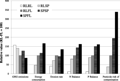
Figure 1. GHG emissions, fossil fuel energy consumption, soil erosion, N and P imbalance ratio and pesticide contamination risk of five background-finishing beef systems of eastern Uruguay, presented as relative to RL–FL system, taken as a reference for comparison (100). (Note: RL: rangeland systems; SP: seeded pasture systems; FL: feedlot systems.)
Download figure:
Standard image High-resolution image
3.7. Trade-offs
Analyzing sustainability of systems should incorporate a broad concept of variables to avoid over-simplification. On the other hand, using too many indicators could generate confusion when discussing results.
We described two global environmental problems (climate change and fossil fuel derived energy consumption) and four variables driving local environmental problems (soil erosion, N and P balance and risk of pesticide contamination). While this is a broad classification, it could help to guide stakeholder's decisions to promote or regulate environmental impact of livestock activities.
There is a trade-off among the six environmental variables analyzed. As systems intensify the use of inputs and increase productivity per unit of resource (land, animals, capital), they perform better in terms of GHG emissions per kg of LW (Capper 2012, Ogino et al 2004) but worse in the other indicators (figure 1).
This trade-off between global and local environmental variables calls for further research in order to define priorities for development. While in order to mitigate a global issue like climate change it could be reasonable to promote beef production in feedlots, in order to mitigate local environmental problems like water contamination through nutrient leaching and pesticides, as well as soil erosion grazing systems are preferred. Also, although rangeland systems seem to be more environmentally friendly systems, they could be undermining soil nutrients in the long term if there is no reposition of N and P extracted.
Quantitative thresholds can give a guide to design more sustainable production systems but the development of these values is still incipient. This analysis gives hints for stakeholders in order to define policies related to food and environment, although further dimensions need to be considered (e.g. biodiversity, water footprint).
4. Conclusions
Environmental impacts of livestock systems have been posed as an important issue in the last decade, since it is placed as one of the largest source of GHG emissions, thus responsible for climate change. Assessing these system's sustainability only through GHG emissions has left behind other issues that should be addressed when looking at agro-ecosystems as a whole and could lead to narrow conclusions. This results show that, as production systems are more intensive on the use of inputs, they enhance productivity and perform better in terms of GHG emissions, but perform worse in terms of energy consumption, soil erosion, generate greater surpluses of P and N, as well as greater pesticides risk of contamination.
Acknowledgments
This research was funded by grants from National Meat Institute—Uruguay (INAC), United Nations Program for Development (PNUD), Ministry of Agriculture, Livestock, and Fisheries—Uruguay (MGAP), and Commission for Scientific Research (CSIC-UDELAR). We are grateful to the farmers and technical advisors who gave us information from their farms to conduct this research.
Footnotes
- 1
Animal unit: a 500 kg live weight cow (Allen et al 2011).