Comparison of Satellite-Derived Land Surface Temperature and Air Temperature from Meteorological Stations on the Pan-Arctic Scale

Abstract

Satellite-based temperature measurements are an important indicator for global climate change studies over large areas. Records from Moderate Resolution Imaging Spectroradiometer (MODIS), Advanced Very High Resolution Radiometer (AVHRR) and (Advanced) Along Track Scanning Radiometer ((A)ATSR) are providing long-term time series information. Assessing the quality of remote sensing-based temperature measurements provides feedback to the climate modeling community and other users by identifying agreements and discrepancies when compared to temperature records from meteorological stations. This paper presents a comparison of state-of-the-art remote sensing-based land surface temperature data with air temperature measurements from meteorological stations on a pan-arctic scale (north of 60° latitude). Within this study, we compared land surface temperature products from (A)ATSR, MODIS and AVHRR with an in situ air temperature (Tair) database provided by the National Climate Data Center (NCDC). Despite analyzing the whole acquisition time period of each land surface temperature product, we focused on the inter-annual variability comparing land surface temperature (LST) and air temperature for the overlapping time period of the remote sensing data (2000–2005). In addition, land cover information was included in the evaluation approach by using GLC2000. MODIS has been identified as having the highest agreement in comparison to air temperature records. The time series of (A)ATSR is highly variable, whereas inconsistencies in land surface temperature data from AVHRR have been found.

1. Introduction

Land surface temperature (LST) is a supporting information source for the generation of the Essential Climate Variable defined by the Global Climate Observing System (GCOS), to support the United Nations Framework Convention on Climate Change (UNFCCC), the World Climate Research Programme (WCRP) and the Intergovernmental Panel on Climate Change (IPCC) [1]. Global climate change, caused by increasing greenhouse gas (GHG) emissions, results significant changes to global ecosystems [2,3].

The arctic environment is highly vulnerable to modifications in the global climate system and currently subject to dramatic changes [4–6]. Predictions are indicating a significant increase of temperature conditions in the arctic regions for the upcoming century [7], which leads to changes in permafrost temperature regimes, snow cover, sea ice, vegetation activities and phenological dynamics [8–11]. Increasing greenhouse gas emissions from thawing permafrost soils will accelerate rising temperature for the upcoming decades, due to positive feedback mechanisms in the global climate system [4,12]. These circumstances are showing the high importance of a consistent and operational monitoring of climate conditions, such as temperature, within the arctic regions. Thus, the problem is the availability of records from meteorological stations, as well as their spatial coverage in these territories. The integration of those ground measurements in climate research, such as modeling and trend analysis, will evoke different problems. The analysis will suffer from the spatial coverage and will not capture the heterogeneity of the arctic climate system. Hence, remote sensing provides a useful tool to retrieve different land surface characteristics over large areas, such as LST [13].

The Data User Element Permafrost (DUE Permafrost), funded by the European Space Agency (ESA), highlighted the needs for a permafrost monitoring system. The aim of this project was to facilitate the cooperation between remote sensing experts and the permafrost science community. To create an observation strategy, various permafrost relevant parameters, such as LST, land cover, subsidence, thermokarst lake changes, soil moisture, etc., which are measurable by satellite systems, were defined. Land surface temperature is one important variable, used as an indicator of the thermal state of the subsurface phenomenon permafrost, which cannot be directly measured with satellite platforms [14]. Hence, there is an increasing demand for integrating LST estimates in arctic research, such as permafrost modeling systems [15].

This paper presents the comparison of state-of-the-art remote sensing-based LST data with air temperature measurements (Tair) for the pan-arctic regions north of 60 degrees latitude. Within this study, we compared LST products from Advanced Very High Resolution Radiometer (AVHRR), Moderate Resolution Imaging Spectroradiometer (MODIS) and (Advanced) Along Track Scanning Radiometer ((A)ATSR) with an in situ Tair database provided by the National Climate Data Center (NCDC). In the context of this paper, the term LST is used for the remote sensing-based temperature information, while Tair refers to the measurement of the meteorological station. The aim is to analyze the agreement between LST and Tair for (1) the complete available period of each product, (2) for the overlapping time period from 2000 to 2005, (3) based on different land cover classes form GLC2000, as well as (4) the spatial distribution of the agreement on the pan-arctic scale.

This paper presents a comparison of LST with Tair records, rather than validation approach. A validation approach of LST requires in situ data, which are based on emissivity measurements of the earth surface using an thermal infrared radiometer (TIR) or comparable systems [13]. Particularly, this paper presents a comparison of two parameters, which have a different physical meaning.

Land surface temperature refers to the radiation properties of the earth surface and determines the intensity of the radiation of long waves emitted by it, which can be detected by aircrafts or satellite-based remote sensing platforms. There are different terms describing the same variable, such as land surface temperature or surface skin temperature. The air temperature or surface air temperature is measured at 1.5–2 m height, where the measurements are done by the contact of the sensor and the surrounding air. Land surface temperature and Tair are correlated to a certain degree, with some drawbacks depending on factors, such as land cover type [16,17].

The comparison is done by using statistical parameters such as the Pearson correlation coefficient (R), the slope (S) and the intercept (INT) with the y-axis of the regression line and the mean difference (MD), also known as bias. The first three parameters were derived by comparing the pixel of the LST data with the corresponding Tair measurements from the meteorological station. Each meteorological station is situated within a pixel of the different remote sensing products. The statistics are based on the scatter cloud derived from the analyzed comparison pairs and time step. The MD is calculated by the difference between Tair and LST divided by the amount of observed time steps. If the MD is negative, the LST detects warmer temperatures than the measured Tair, and vice versa[13].

2. Data

2.1. Remote Sensing Data

2.1.1. AVHRR Polar Pathfinder Land Surface Temperature

The AVHRR Polar Pathfinder product covers the polar regions of the northern and southern hemisphere with a spatial coverage north of 48° and south of 53° in latitude and have been used for several studies [18–22]. The product includes five AVHRR channels, covering one visible, one infrared and three thermal infrared bands, as well as surface albedo, skin surface temperature, solar zenith angle, satellite elevation angle, azimuth angle, surface type and a cloud mask. The product covers the time period from July 1981 to June 2005 and is based on data from NOAA-7, 9, 11, 14 and 16. It is a twice-daily dataset acquiring the imagery at 4 a.m. and 2 p.m. in the northern hemisphere. For this study, only daytime LST estimates have been used. The data is available in EASE-Grid projection (Equal Area Scalable Earth-Grid) with spatial resolution of 5 km [23]. The LST is extracted by two algorithms, which utilize the brightness temperature of spectral channels 4 (10.3–11.3 μm) and 5 (11.5–12.5 μm) [24].

The data quality of the AVHRR Polar Pathfinder product is influenced by an orbital drift of each NOAA satellite during their lifetime, which causes a shift of the equator crossing time to the afternoon. This orbital drift evokes a cooling effect to the LST estimates. The effect was found to be stronger on the southern hemisphere and non-vegetated regions [25,26]. Since this study focuses on the cold regions of the northern hemisphere, the effect of the orbital drift is negligible and not part of its scope.

2.1.2. MODIS Land Surface Temperature (MOD11C1, MYD11C1)

The LST products from MODIS Terra and Aqua are widely used for remotely sensed temperature research such as [17,27–35]. The product covers a range of different datasets ranging from 1 km to 0.05° (approx. 5.6 km at equator; CMG—Climate Modeling Grid) spatial resolution, as well as daily, eight-day and monthly temporal resolution. Both satellite platforms have sun-synchronous orbits. MODIS Terra acquires the data at 10:30 a.m./p.m. (daytime/nighttime), whereas MODIS Aqua collects the imagery at 1:30 p.m./a.m. (daytime/nighttime) [36]. For this study, daily MODIS LST products MOD11C1 and MYD11C1 (Version 5) with a resolution of 0.05° were used.

The MODIS LST products (MOD11C1, MYD11C1) were derived from MOD11B1, which has a daily resolution with 6 km pixel size in sinusoidal projection. This product is developed from algorithms defined in [37], whereby the temperature and emissivity extraction from 7 of 16 emissivity bands from MODIS that cover the thermal infrared spectrum (TIR) are described. In detail, the bands 20 (3.66–3.84 μm), 22 (3.93–3.98 μm), 23 (4.02–4.08 μm), 29 (8.40–8.70 μm), 31 (10.78–11.28 μm), 32 (11.77–12.27 μm) and 33 (13.18–13.48 μm) were used for the approach. Compared to the other channels from MODIS, these channels, also known as window bands, remain virtually unaffected by changes in temperature and amount of water vapor within elevations above 9 km [37].

The retrieval of LST from MODIS is based on various input parameters, which were also available as individual products. In general, only swaths, which have a valid Level 1B radiance in channels 31 (10.78–11.28 μm) and 32 (11.77–12.27 μm), are over land (including water bodies) and are acquired under clear sky conditions, in addition to being used to derive LST information. The extraction is done by a classification-based algorithm developed by [38], in which emissivity estimates from band 31 and band 32 are used. Additional input parameters, such as cloud mask (MOD35_L2), atmospheric profiles (MOD07_L2), geo-location (MOD03), land cover (MOD12Q1) and snow cover (MOD10_L2), are integrated into the algorithm.

2.1.3. Land Surface Temperature from AATSR

The LST product by the European Space Agency (ESA), which was provided for this study, was derived using ATSR-1 on ERS-1, ATSR-2 on ERS-2 and AATSR on ENVISAT earth observation data. All satellites have sun-synchronous orbits, where ERS-1 and ERS-2 acquire data at 10:30 a.m. and ENVISAT at 10 a.m. [39,40]. The LST product is produced using a nadir-split window approach calculating brightness temperature from 11 μm and 12 μm described in [41]. Coefficients depending on the atmospheric water vapor, the viewing angle and the land-surface emissivity are considered in the algorithm [41–43]. The ESA is planning to develop a GlobTemperature program based on the data from ERS-1 and 2, ENVISAT and upcoming missions during the next year. A first user workshop, to address the user’s needs for a global LST dataset, was held in Edinburgh in mid-2012 [44].

This global product covers the time period from August 1991 to December 2009 with a spatial resolution of 9.28 km in sinusoidal projection. The product has monthly resolution, where each month is covered by approximately 430 orbits at a resolution of 1 km. The final product resolution of 9.28 km is based on a composite and consists of pixels marked as land and cloud-free. The discrimination between day and nighttime data was done using sun elevation information [40,45].

Some issues about the data quality due to anomalies of the sensors during their data acquisitions times were identified. In May 1992, the 3.7 μm channel from ATSR-1 was lost. There were no data between January and June 1996 due to problems with the downlink and the tape capacity followed by a reduced swath within the visible channels since June 2001. AATSR onboard of ENVISAT suffered from a spectral drift in the 0.55-μm channel from December 2005 to December 2006, which was corrected a priori by a model defined by [46]. Since all three sensors are using identical thermal infrared channels, which are used deriving LST information, it has to be mentioned that all of the sensors are onboard of three different platforms with individual orbits and acquisition times. This is an important point to highlight in a product combined from similar but unique sources [45].

2.2. Global Surface Summary of Day Data—Version 7

The comparison of the daily and monthly remote sensing-based LST estimates with ground measurements were done using the Global Surface Summary of Day Data (GSOD), an in situ database from NOAA (National Oceanic and Atmospheric Administration) National Climate Data Center (NCDC). The product provides daily information about 18 meteorological parameters, such as Tair (min, mean and max), wind speed, wind gust, and amount of precipitation, from over 8,000 stations worldwide. This GSOD dataset is based on the Integrated Surface Database (ISD), an initiative developed in 1998 by a cooperation of NCDC, US Air Force and US Navy. The aim of this program is to provide hourly consistent climate measurements back to the 19th century to address the needs of global climate studies [47–49].

The database of the Global Summary of Day Data is updated on a daily frequency. In general, the majority of the temporal availability of the meteorological stations goes back to the 1970s, for some cases even back to the 1930s and earlier. There are known issues about the data availability for some regions, which could be interrupted for some time periods due to data restrictions or communication problems. However, all available daily data records are based on a minimum of four observations per day. The data quality is automatically controlled and corrected, which prevents larger data gaps within the database [49].

3. Methodology

The comparison of remote sensing-based LST estimates and Tair records from the meteorological station is performed with six processing steps:

(1)

Extraction of meteorological stations on pan-arctic scale (above 60 degrees north).

(2)

Identification of geographic location of meteorological stations and extraction of data from pixels in remote sensing-based LST products.

(3)

Comparison of LST and Tair time series for the whole temporal coverage of each product.

(4)

Reduction of both databases to the overlapping time period of the remote sensing products (2000–2005).

(5)

Inter-annual comparison of LST and Tair data based on the overlapping time period.

(6)

Link of the results to land cover classes extracted for each meteorological stations based on GLC2000 (Global Land Cover 2000).

• The extractions of the meteorological stations, which are situated north of 60 degrees, are done by metadata file, which was provided by the NCDC. This file includes additional information for each station, such as station ID, starting time of acquisition, geographic coordinates, country and measured parameters. This extraction results in over 600 stations suitable for this analysis. After an automated consistency check, identifying missing daily data, the data gaps where filled to create a consistent database. Meteorological stations, which have shown a significant number of missing data, were not used for this study.
• To develop a comprehensive validation database, the geographic coordinates of each of the selected meteorological stations was extracted from the metadata and applied to the remote sensing time series product. Afterwards it was possible to convert the pixel stack from the LST products, which are including each time step, into a single vector. For each meteorological station, a matrix was developed, which included the time, the LST that was based on the remote sensing data, and the Tair values.
• In a first step, the remote sensing-based LST was compared to Tair measurements for the complete time series of each product (Section 4.1). Only daytime temperature information was used in this study. This analysis should give an impression about the agreement between both parameters.
• To derive a detailed insight in the comparison and to assure the comparability of this study, the overlapping period of the remote sensing products (2000–2005) was analyzed (Section 4.2).
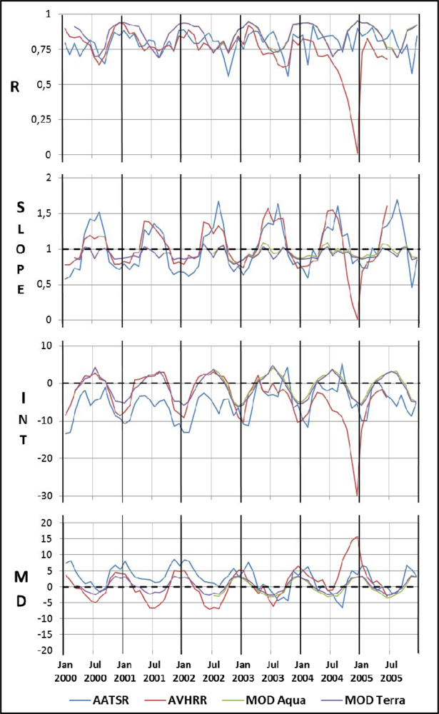
• For this time period, the inter-annual variability between LST and Tair were analyzed, using different statistical parameters, such as the Pearson correlation coefficient (R), the slope (S) and the intercept of the regression line (I), as well as the mean difference (MD).
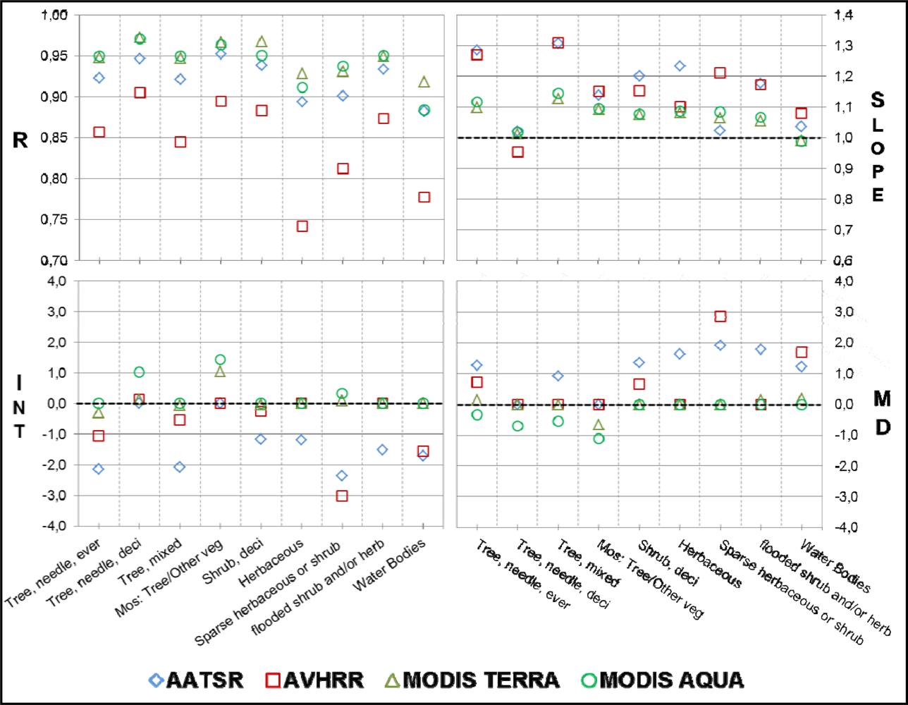
• Prior to the inter-annual variability by comparing LST and Tair time series information, the results were linked to land cover units (Sections 4.3 and 4.4). The goal was to provide information about land cover classes, which are showing the highest variability and discrepancies between remote sensing and ground temperature measurements. The aim was to use the most recent global land cover product GlobCover 2009, developed by ESA [50]. Unfortunately, this classification is not suitable for this analysis, since the land cover class “needle-leaved deciduous forest” (80) does not appear in the final product. The reason for that is that this class needs a seasonal observation from a remote sensing satellite, which was not sufficient for this classification [50]. Thus, the Global Land Cover Classification 2000 (GLC2000), produced by the Joint Research Centre (JRC), was used for this study. This classification is based on satellite data from VEGETATION on SPOT-4 and uses the standardized Land Cover Classification System (LCCS) developed by FAO (Food and Agriculture Organization) as land cover legend [51]. A brief overview of the methodology is shown in Figure 1.

4. Results and Discussion

4.1. Correlation of Remote Sensing-Based LST Estimates with Tair Measurements

The following chapter presents the results from the comparison of LST from (A)ATSR (monthly mean values), AVHRR and MODIS (both daily mean values) with daily mean in situ measurements from meteorological stations. Each plot shows the correlation of the comparison based on the time series of each product with Tair data (Figure 2). The density cloud plot is divided into temperatures above and below 0 degree Celsius (°C), while showing the corresponding regression line as well as the Pearson’s correlation coefficient (R).

The LST product from (A)ATSR covers the time period of 1991 to 2009 with a monthly temporal resolution. When compared to Tair measurements, a correlation of R = 0.89 is achieved. The remote sensing data detects colder temperatures than those measured on the ground within a range of 0 to 15 °C. Above 15 °C, the opposite becomes visible. The agreement between LST and Tair for temperatures above 0 °C are described by a correlation coefficient R = 0.75. Observing the negative temperature range, LST is showing colder temperatures until approximately −30 °C. Below this value, LST appears to be warmer. The negative temperature range results in a correlation coefficient of R = 0.81. Thus, higher correlations are found for temperatures below the freezing point.

The LST estimates from the AVHRR Polar Pathfinder dataset results in an overall correlation of R = 0.9, which is comparable to the correlation coefficient of (A)ATSR. However, AVHRR has a larger temporal coverage (1981–2005) and has a daily temporal resolution. Similar to (A)ATSR, LST from AVHRR results in colder temperatures compared to the corresponding Tair measurements within a temperature range from 0 and 5 °C and the opposite above this range, causing a correlation coefficient of R = 0.74. For temperature values below 0 °C, (A)ATSR and AVHRR are showing similarities. Until a value of −30 °C, LST is slightly colder than Tair. Afterwards, LST values are warmer than the corresponding Tair values. The correlation coefficient is R = 0.82.

The overall correlation coefficient of MODIS Terra and Aqua is higher than for (A)ATSR and AVHRR (R = 0.95). However, MODIS Terra and Aqua are covering a shorter time period. The correlation of temperature above 0 °C shows a slight overestimation with a very close fit of the regression line to the 1:1 line. The correlation coefficient is higher (R = 0.80) than for (A)ATSR and AVHRR. The correlation of negative temperature is very high with R = 0.92, which also results in a very close fit of the regression line and the 1:1 line.

In summary, MODIS Terra and Aqua LST estimates display a higher correlation when compared to Tair records, followed by (A)ATSR and AVHRR. The concentration of the point density within the scatter cloud is close to the 1:1 line, which is also the case for AVHRR. Values around 0 °C and slightly warmer seems to show the highest concentration of compared data pairs, except for (A)ATSR. AVHRR and (A)ATSR show outliers at 0 °C of the x-axis ranging down to −60 °C of the y-axis. These artifacts may be caused by the cloud and ice detection algorithm of the products. Since temperature conditions in the lower atmosphere (top of clouds) are much lower [52] than the temperature of snow or ice covered surfaces, confusion between cloud and ice detection during the winter season could cause this problem.

In general, LST appears to result in warmer values compared to Tair within the positive temperature range for all remote sensing products. This problem exists due to the fact that LST and Tair are based on different physical processes [16], as described in the introduction. Land surface temperature is warmer in positive temperature ranges than Tair, which is measured at a height of 2 m, as standardized for meteorological stations. Increased solar irradiance (e.g., during the summer month), causes higher land surface temperatures, thereby leading to this overestimation [53].

4.2. Inter-Annual Variability of LST Estimates for the Time Period between 2000 and 2005

This chapter highlights the inter-annual variability of different statistical parameters extracted by the comparison of LST and Tair. Due to the large amount of data, each time step represents the median of all measurements. Figure 3 gives an overview of the variation between the time periods of 2000 to 2005, which is the overlapping time period of the used remote sensing products and enables a refined comparability.

The correlation coefficient (R) describes the variance of the point cloud around the regression line, showing the dependencies between LST and Tair. The variability of R during the time period of 2000 to 2005 is quite similar for all products, with the majority ranging between 0.6 and 0.9 during the yearly cycle. Higher correlations can be found in the winter season and lower during the summer month. An explanation could be the higher turbulences between land surface and atmosphere in the summer month in comparison to the winter month with lower incoming solar radiation [34]. AATSR is showing the highest inter-annual dynamics compared to the other products. Since 2003, AATSR is not capturing the yearly dynamics of the other products. Land surface temperatures from MODIS are showing similar inter-annual variations when compared to Tair measurements. The dynamics of AVHRR are comparable to the variability identified for MODIS. However, AVHRR is resulting in larger amplitudes of the dynamics.

In general, MODIS results in consistent inter-annual dynamics in contrast to more variations identified in AATSR and data inconsistencies for some months in the AVHRR product. A drop of the correlation coefficient is found at the end of 2004 for the AVHRR data. This might be due to the data quality, consistence of acquired data and algorithm processing chain. Known issues include problems with the scan motor on NOAA-16, which causes sporadic, irregular shifts within the derived spectral information [23], as well as the orbital drift of the NOAA satellites, which in turn causes a delay in overflying time [25,26]. Another reason could be that the data from AATSR has a monthly temporal resolution. The number and the time of observations may vary from month to month during this time period.

The statistical parameters Slope (S) and Intercept (Int) describe the dynamics of the point clouds. A slope of 1 exists when the regression line is parallel to the line of best fit (x equals y). If the intercept equals 0, the regression line and the line of best fit are congruent. In combination with the correlation coefficient, which describes the variance around the regression line, these three statistical parameters allow for a detailed interpretation comparing LST and Tair. AVHRR and AATSR display large variability observing the slope. During the wintertime, the products have resulting slopes of −0.5, which is an indicator of lower dynamics during this time of the year. In the summer months, higher dynamics can be found by slopes with the value of 1.5. MODIS LST is very close to slopes of 1, which indicates low dynamics during the year. This is applicable during the summer season, while the winter season is showing fairly lower slopes of 0.8.

The statistical parameter Intercept (Int) is congruent for the AVHRR and MODIS data for the years 2000–2002. AATSR shows the same dynamics, but is fairly lower. For the year 2003 and beyond, AATSR and AVHRR have the same variability, while MODIS continues the dynamic patterns of the previous years. The decrease of the slope and intercept statistic values for the AVHRR at the end of 2004 data also becomes visible.

The relation of the correlation coefficient, the slope as well as the intercept indicates that LST was lower than the equivalent Tair during the wintertime for all LST products. This assumption is based on slopes, which are below 0 while showing a negative intercept with the y-axis. The summer season is characterized by slopes above a value of 1 in combination with positive intercepts, which indicates an overestimation of the positive temperature range and an underestimation of negative temperatures.

The correlation coefficient during the summer is lower in comparison to the winter month, indicating higher variances in differences between LST and Tair. In general, the diurnal temperature magnitude is lower in winter as in the summer season. This causes larger variations between day and night temperatures [34,54]. It needs to be mentioned that the diurnal cycle is also influenced by different moisture conditions of the earth surface [31], as well as water vapor within the lower atmosphere [34]. Nevertheless, the findings illustrate lower dynamics between LST and Tair for negative temperatures. The positive temperature range, influenced by larger diurnal temperature differences, results in higher divergences between LST and Tair measurements.

The mean difference (MD) is an indicator describing whether remote sensing-based LST data detects warmer or colder temperature in comparison to Tair. If the MD is negative, the LST detects warmer temperatures than the measured Tair, and vice versa[13]. All products show a similar inter-annual variability. The MODIS product is close to 0 for the whole time period. AVHRR is showing similar bias values in comparison to MODIS. In detail, higher differences between MODIS and AVHRR are found in the summer than during the winter season, which have been recently identified by [55]. AATSR detects solely colder temperatures for the first three years, which is followed by an adaption to the seasonal cycle of the other products, but still higher variations.

In general, the summer months are showing a slightly negative bias, which indicates that the land LST estimation results in warmer temperature than the measured Tair. For the winter season, the opposite is found. The positive mean difference values are caused by colder LST estimates than measured by the meteorological station at 2 m height. The lowest bias can be found for spring and autumn, which was also found for the other statistical parameters.

The observed variability and derivations between LST and Tair could be caused by the different pixel sizes of the products. MODIS and AVHRR have a spatial resolution of approx. 5 km, whereas AATSR has a resolution of about 9 km. This is changing the influence of the heterogeneity of the land surface in the LST pixel. Moreover, the LST values from AATSR are based on monthly mean. Hence, a comparison to daily values from MODIS and AVHRR is a challenging issue.

The findings are indicating low agreements between LST and Tair during peak temperatures events for both positive and negative ranges, which are found in summer and winter. Besides this, spring and autumn, which are characterized by moderate temperatures and diurnal differences, are showing a higher agreement and a lower bias between LST and Tair.

In summary, MODIS seems to shows the best fit between LST and Tair. Data from AATSR is affected by high inter-annual variability, which reduces the consistency of the dataset. Comparing LST from AVHRR with Tair, inconsistencies are also found in the time series, such as the drop of in the end of 2004.

4.3. Comparison of Land Surface Temperature and Air Temperature for Selected Land Cover Classes

The statistical parameters comparing LST with Tair estimates are linked to land cover classes for each station. As it was done in Section 4.2, only the median is displayed in Figure 4. The land cover information was derived using GLC2000 global land cover classification [51]. Only classes, including more than 20 stations, are shown below (Figure 4). The standard deviation of each data point is shown in

Table 1. Standard deviation of the statistical parameters correlation coefficient and mean difference for selected land cover classes.

Land Cover	AATSR	AVHRR	MOD Terra	MOD Aqua	ø	AATSR	AVHRR	MOD Terra	MOD Aqua	ø
	R					Mean Difference
tree, needle, ever	0.38	0.29	0.29	0.33	0.32	2.66	2.70	1.49	1.78	2.16
tree, needle, deci	0.49	0.48	0.50	0.50	0.49	1.51	1.46	1.17	1.51	1.41
tree, mixed	0.39	0.37	0.36	0.38	0.38	1.76	2.86	0.98	1.19	1.70
mos: tree/other veg	0.46	0.42	0.43	0.45	0.44	1.44	1.59	0.82	1.21	1.26
shrub, deciduous	0.42	0.30	0.24	0.35	0.33	3.04	3.96	1.59	1.75	2.59
herbaceous	0.45	0.41	0.40	0.42	0.42	3.03	3.96	1.52	1.72	2.56
sparse herb or shrub	0.33	0.24	0.27	0.29	0.28	2.05	3.13	1.47	1.75	2.10
flood shrub/herb	0.42	0.38	0.41	0.44	0.41	2.13	1.87	1.22	1.13	1.59
water bodies	0.42	0.35	0.38	0.40	0.39	2.92	3.20	1.56	1.65	2.33

.

The correlation coefficient R was above 0.7 for all selected classes and products, which is an indicator for a good agreement between LST and Tair. However, MODIS showed the highest correlation for all classes (>0.9) while AVHRR results in lower coefficients for all classes. The range between the correlation coefficient of the products is low for classes, which are dominated by forest classes. Land cover units characterized by lower vegetation and sparse vegetation were showing a higher range of R-values. From the perspective of land cover classification, forest classes were defined as stable, whereas shrub land and herbaceous vegetation classes, characterized by a mixture of plant species, were known to be heterogeneous landscape units [56]. Additionally, the heterogeneity is also an effect of the large pixel size of the remote sensing-based LST products, affecting the estimation of the LST for specific land cover types [57].

The majority of the land cover classes resulted in slopes above 1, except for water bodies, as well as needle-leaved deciduous trees, one of the dominant vegetation types in Siberia. Both land cover types resulted in slope values close to 1, indicating a nearly identical dynamic between the observed and the measured variables. Slopes above 1 resulted if LST was showing higher dynamics than Tair. In combination with the intercept, it is possible to derive information about whether LST is warmer or colder than the corresponding Tair measurements.

Land cover types such as needle-leaved evergreen forest, mixed forest, mosaic forest with other natural vegetation, shrubs, herbaceous and sparse vegetation, as well as flooded areas and water bodies, resulted in slopes above 1 and negative intercepts. This indicated that LST is warmer than Tair in positive and negative temperature range. In detail, the remote sensing sensors detect warmer temperature in positive temperature range and colder temperatures in negative range. For all these classes, AATSR and AVHRR had a stronger influence over this circumstance. Good agreement of LST and Tair was found for the needle-leaved deciduous forest, mosaic forest and other vegetation, sparse vegetation and flooded areas.

The statistical parameter mean difference is zero or positive for non-forest classes. These land cover types also showed the highest range between the products, where AATSR showed the highest values for this statistical parameter. The positive mean difference values thus indicate that LST estimates colder temperatures than those measured in the field. In comparison, the forest classes showed a negative bias, thereby indicating that warmer temperatures have been detected by the remote sensing data. In general, MODIS results in low mean difference values, which suggests the measured LST estimates to be close to the Tair (see Section 4.2). The needle-leaved deciduous forest land cover class, which is one of the major vegetation types, showed high agreement between LST and Tair by a low bias for all products.

The standard deviations of the correlation coefficient as well for the mean difference for each product and land cover type are shown in Table 1. AATSR results had the highest standard deviation values for the correlation coefficient. For the mean difference, AVHRR had the highest standard deviation, while MODIS Terra showed the lowest. The ranges of the standard derivations for the slope, which are not shown in the table, were similar for all products and land cover classes (0.44–0.62). In contrast, the correlation coefficient, intercept (not shown in Table 1) and mean difference were characterized by larger derivation of the standard deviation between the products for the selected land cover classes. The forest classes showed the lowest differences for the standard deviations, particularly for the mean difference. Moreover, sparse vegetated classes, as well as herbaceous and shrub lands, had larger discrepancies in standard deviation values. As discussed in Section 4.3, the heterogeneity of the land surface has a major impact on the derived agreement between LST and Tair. Thus, comparing LST and Tair for different land cover units, heterogeneous land cover units seem to be rather variable and differ from more stable classes, such as tree cover classes. Additionally, the coarse pixel size of the LST products enhances the effect of heterogeneity [55].

In general, MODIS LST estimates resulted in the lowest standard deviations when compared to AATSR and AVHRR. As it was identified in Sections 4.1 and 4.2, the LST estimates from MODIS showed the agreement with Tair measurements and also had the lowest magnitude variability within the observed time series. Thus, the MODIS products are defined as consistent and having the highest confidence compared to the other products.

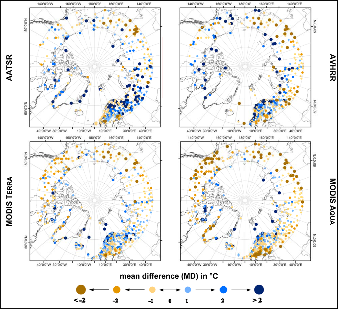
4.4. Pan-Arctic Perspective of the Mean Difference for the Time Period of 2000–2005

Figure 5 presents the mean difference for all meteorological stations, covering the pan-arctic circle. The values of the legends are ranging from −2 °C to 2 °C (Note: higher positive and negative values might occur). The colors are ranging from orange (warmer) to blue (colder). The size of the circles provides information about the height of the mean difference. Larger circles indicate higher mean differences in both directions, positive and negative. In general, maritime-dominated regions, such as coastal areas, indicate that the remote sensing-based LST detects colder temperature conditions than those acquired by the meteorological stations. Furthermore, stations within a continental climate regime show that LST is warmer than Tair. This is the case for all products. Moreover, the magnitude of positive and negative peaks is higher in continental regions, which indicates higher variations within the LST retrieval. The stability of temperature conditions in maritime regions around the arctic coastline in comparison to continental areas have been highlighted by [58].

Comparing the products, AATSR and AVHRR showed larger values in both directions than MODIS, indicating a higher bias especially in Europe and the western part of Russia. AATSR detects colder temperatures over large areas when compared to in situ measurements. AVHRR and MODIS Terra are also showing this phenomenon in these areas. However, the biases are quite low. MODIS Aqua does not reflect these findings for Europe and the western part of Russia. The mean difference values were negative, which indicates that LST is warmer than Tair. These findings are reasonable, since the acquisition time of MODIS Aqua is in the afternoon, which causes warmer temperatures during the day. Thus, the solar irradiance has changed during both acquisition times, causing an increase in LST. It is expected that AVHRR also shows the same bias than MODIS Aqua, since AVHRR also acquires the satellite data during the afternoon. One reason for these dissimilarities could be the orbital drift of the NOAA satellite, which causes a delay in overflying time. Since the data is acquired later during the day, the temperature conditions could already decline towards the late afternoon. Hence, the temperature conditions could be similar to those during the morning time (MODIS Terra, AATSR). In the far eastern parts of Russia, all products showed a similar bias. However, some differences in the height of mean difference values can be found when AVHRR is compared with the other products. The territories of North America are showing the same patterns between AATSR and AVHRR. Moreover, a different distribution of the mean difference values was found for both MODIS products. In contrast to AATSR and AVHRR, the LST estimates were detected to be warmer than Tair (negative MD). This is already the case for the morning data (MODIS Terra) and increases during the afternoon, which can be found for the MODIS Aqua data.

5. Conclusion and Outlook

Land surface temperature information (LST) from AVHRR (Advanced Very High Resolution Radiometer), MODIS (Moderate Resolution Imaging Spectroradiometer) and (A)ATSR ((Advanced) Along Track Scanning Radiometer) were compared to in situ air temperature measurements (Tair) from the National Climate Data Center (NCDC). The quality characteristics are addressed to the climate modeling community, as well as other climate-related research groups.

MODIS LST has shown the highest agreement in comparison to Tair. (A)ATSR and AVHRR tend to detect warmer and colder temperatures for the positive and negative temperature ranges. MODIS is showing minor overestimations in the positive temperature range. (A)ATSR and AVHRR indicate outliers around the freezing point. These artifacts are referred to errors in the processing chain, when differentiating between clouds and snow, as well as ice-covered regions.

High agreements between LST and Tair can be found for the winter season with a decline towards the summer months [55]. AATSR has the highest inter-annual variability. Some issues can be found for AVHRR, induced by a decrease of the agreement at the end of 2004. The bias of MODIS LST is close to zero for the entire time, whereas larger variability is found for AATSR and AVHRR.

High correlations are found for all land cover classes. The ranges of the correlation coefficient between the products are low for tree cover classes. Heterogeneous land surfaces, such as herbaceous and shrub lands, result in higher discrepancies. MODIS LST results in the lowest bias, emphasizing the quality of the product. Differences between maritime and continental areas are found. The results have shown coastal regions to be characterized by positive mean difference values, indicating LST to be colder than Tair. Continental areas are characterized by an overestimation of the Tair.

Coarse resolution LST information was compared to point measurements on the ground. The comparison between pixel and point values can bring uncertainties to the analysis caused by land cover, snow cover, topography, soil moisture and surface water, etc.[13]. The arctic regions are characterized by a high density of thermokarst lakes, non-vegetated surfaces (rocks), as well as snow and ice, which have a strong influence over the emission characteristics of the earth’s surface. Additionally, the diurnal cycle is a challenging issue which needs to be addressed in LST studies. Investigations are carried out by combining daytime and nighttime LST observations, which have shown the potential to reduce the discrepancies [15].

As daily and monthly mean temperatures are compared in this study, future investigations need to be carried out addressing the actual daytime of the observed LST and measured Tair. Daily LST information from (A)ATSR might become available within the upcoming GlobTemperature program by ESA (European Space Agency) [45]. The Integrated Surface Database (ISD), known as Integrated Surface Hourly (ISH), provides, besides the daily mean, information about the exact time of the day of the acquired Tair. Thus, a direct connection between the overpass time of the satellite and the acquired Tair can be achieved [59]. This would improve the analysis of comparing remote sensing-based LST and Tair measurements from meteorological stations.

References

1. GCOS. Supplemental Details to the Satellite-Based Component of the “Implementation Plan for the Global Observing System for Climate in Support of the UNFCCC (2010 Update). 2011. Avaiable online: http://www.wmo.int/pages/prog/gcos/documents/SatelliteSupplement2011Update.pdf (accessed on 28 February 2013).
2. Overpeck, J.; Hughen, K.; Hardy, D.; Bradley, R.; Case, R.; Douglas, M.; Finney, B.; Gajewski, K.; Jacoby, G.; Jennings, A.; et al. Arctic environmental change of the last four centuries. Science 1997, 278, 1251–1256. [Google Scholar]
3. Chapin, F.S.; Sturm, M.; Serreze, M.C.; McFadden, J.P.; Key, J.R.; Lloyd, A.H.; McGuire, A.D.; Rupp, T.S.; Lynch, A.H.; Schimel, J.P.; et al. Role of land-surface changes in arctic summer warming. Science 2005, 310, 657–660. [Google Scholar]
4. Moritz, R.E.; Bitz, C.M.; Steig, E.J. Dynamics of recent climate change in the Arctic. Science 2002, 297, 1497–1502. [Google Scholar]
5. Grace, J.; Beringer, F.; Laszlo, N. Impacts of climate change on the tree line. Ann. Bot. 2002, 90, 537–544. [Google Scholar]
6. Nelson, F.E. (Un)frozen in Time. Science 2003, 299, 1673–1675. [Google Scholar]
7. Kaplan, J.O.; New, M. Arctic climate change with a 2 °C global warming: Timing, climate patterns and vegetation change. Climatic Change 2006, 79, 213–241. [Google Scholar]
8. Post, E.; Forchhammer, M.C.; Bret-Harte, M.S.; Callaghan, T.V.; Christensen, T.R.; Elberling, B.; Fox, A.D.; Gilg, O.; Hik, D.S.; Høye, T.T.; et al. Ecological dynamics across the Arctic associated with recent climate change. Science 2009, 325, 1355–1358. [Google Scholar]
9. Hinzman, L.D.; Stow, D.A.; Hope, A.; McGuire, D.; Verbyla, D.; Gamon, J.; Huemmrich, F.; Houston, S.; Racine, C.; Sturm, M.; et al. Remote sensing of vegetation and land-cover change in Arctic Tundra ecosystems. Remote Sens. Environ. 2004, 89, 281–308. [Google Scholar]
10. Myneni, R.B.; Keeling, C.D.; Tucker, C.J.; Asrar, G.; Nemani, R.R. Increased plant growth in the northern high latitudes from 1981 to 1991. Nature 1997, 386, 698–702. [Google Scholar]
11. Romanovsky, V.; Burgess, M.; Smith, S.; Yoshikawa, K.; Brown, J. Permafrost temperature records: Indicators of climate change. EOS Trans. AGU 2002, 83, 589–594. [Google Scholar]
12. Serreze, M.C.; Walsh, J.E.; Osterkamp, T.E.; Dyurgerov, M.; Romanovsky, V.E.; Oechel, W.C.; Morison, J.; Zhang, T.; Barry, R.G. Observational evidence of recent change in the northern high-latitude environment. Climatic Change 2000, 46, 159–207. [Google Scholar]
13. Hachem, S.; Duguay, C.R.; Allard, M. Comparison of MODIS-derived land surface temperatures with ground surface and air temperature measurements in continuous permafrost terrain. Cryosphere 2012, 6, 51–69. [Google Scholar] [Green Version]
14. Bartsch, A.; Wiesmann, A.; Strozzi, T.; Schmullius, C.; Hese, S.; Duguay, C.; Heim, B.; Seifert, F.M. Implementation of a Satellite Data Based Permafrost Information System—The DUE Permafrost Project. Proceedings of ESA Living Planet Symposium 2010, Bergen, Norway, 28 June–2 July 2010.
15. Soliman, A.; Duguay, C.; Saunders, W.; Hachem, S. Pan-arctic land surface temperature from MODIS and AATSR: Product development and intercomparison. Remote Sens. 2012, 4, 3833–3856. [Google Scholar]
16. Jin, M.; Dickinson, R.E. Land surface skin temperature climatology: Benefitting from the strengths of satellite observations. Environ. Res. Lett. 2010. [Google Scholar] [CrossRef]
17. Mildrexler, D.J.; Zhao, M.; Running, S.W. A global comparison between station air temperatures and MODIS land surface temperatures reveals the cooling role of forests. J. Geophys. Res. 2011, 116, 1–15. [Google Scholar]
18. Maslanik, J.; Fowler, I.C.; Key, I.J.; Scambos, T.E.D.; Son, T.H.; Emeryl, V. AVHRR-based polar pathfinder products for modeling applications. Ann. Glaciol. 1997, 25, 388–392. [Google Scholar]
19. Green, R.M.; Hay, S.I. The potential of Pathfinder AVHRR data for providing surrogate climatic variables across Africa and Europe for epidemiological applications. Remote Sens. Environ. 2002, 79, 166–175. [Google Scholar]
20. Sobrino, J.A.; Julien, Y.; Morales, L. Multitemporal analysis of PAL images for the study of land cover dynamics in South America. Glob. Planet. Chang. 2006, 51, 172–180. [Google Scholar]
21. Julien, Y.; Sobrino, J.A.; Verhoef, W. Changes in land surface temperatures and NDVI values over Europe between 1982 and 1999. Remote Sens. Environ. 2006, 103, 43–55. [Google Scholar]
22. Ouaidrari, H.; Goward, S.N.; Czajkowski, K.P.; Sobrino, J.A.; Vermote, E. Land surface temperature estimation from AVHRR thermal infrared measurements. An assessment for the AVHRR Land Pathfinder II data set. Remote Sens. Environ. 2002, 81, 114–128. [Google Scholar]
23. Fowler, C.; Maslanik, J.; Haran, T.; Scambos, T.; Key, J.; Emery, W. AVHRR Polar Pathfinder Twice-Daily 5 km EASE-Grid Composites V003. Avaiable online: http://nsidc.org/data/docs/daac/nsidc0066_avhrr_5km.gd.html (accessed on 15 March 2012).
24. Key, R.; Collins, J.B.; Fowler, C.; Stone, R.S. High-latitude surface temperature from thermal satellite data. Remote Sens. Environ. 1997, 61, 302–309. [Google Scholar]
25. Gleason, A.C.R.; Prince, S.D.; Goetz, S.J.; Small, J. Effects of orbital drift on land surface temperature measured by AVHRR thermal sensors. Remote Sens. Environ. 2002, 79, 147–165. [Google Scholar]
26. Julien, Y.; Sobrino, J.A. Correcting AVHRR Long Term Data Record V3 estimated LST from orbital drift effects. Remote Sens. Environ. 2012, 123, 207–219. [Google Scholar]
27. Hengl, T.; Heuvelink, G.B.M.; Perčec Tadić, M.; Pebesma, E.J. Spatio-temporal prediction of daily temperatures using time-series of MODIS LST images. Theor. Appl. Climatol. 2012, 107, 265–277. [Google Scholar]
28. Guangmeng, G.; Mei, Z. Using MODIS land surface temperature to evaluate forest fire risk of northeast China. IEEE Geosci. Remote Sens. Lett. 2004, 1, 98–100. [Google Scholar]
29. Julien, Y.; Sobrino, J. The Yearly Land Cover Dynamics (YLCD) method: An analysis of global vegetation from NDVI and LST parameters. Remote Sens. Environ. 2009, 113, 329–334. [Google Scholar]
30. Liu, Y.; Hiyama, T.; Yamaguchi, Y. Scaling of land surface temperature using satellite data: A case examination on ASTER and MODIS products over a heterogeneous terrain area. Remote Sens. Environ. 2006, 105, 115–128. [Google Scholar]
31. Langer, M.; Westermann, S.; Boike, J. Spatial and temporal variations of summer surface temperatures of wet polygonal tundra in Siberia—Implications for MODIS LST based permafrost monitoring. Remote Sens. Environ. 2010, 114, 2059–2069. [Google Scholar]
32. Hulley, G.C.; Hook, S.J. Intercomparison of versions 4, 4.1 and 5 of the MODIS Land Surface Temperature and Emissivity products and validation with laboratory measurements of sand samples from the Namib desert, Namibia. Remote Sens. Environ. 2009, 113, 1313–1318. [Google Scholar]
33. Zhong, L.; Ma, Y.; Su, Z.; Salama, M.S. Estimation of land surface temperature over the Tibetan Plateau using AVHRR and MODIS data. Adv. Atmos. Sci. 2010, 27, 1110–1118. [Google Scholar]
34. Zhang, W.; Huang, Y.; Yu, Y.; Sun, W. Empirical models for estimating daily maximum, minimum and mean air temperatures with MODIS land surface temperatures. Int. J. Remote Sens. 2011, 32, 9415–9440. [Google Scholar]
35. Crosson, W.L.; Al-Hamdan, M.Z.; Hemmings, S.N.J.; Wade, G.M. A daily merged MODIS Aqua-Terra land surface temperature data set for the conterminous United States. Remote Sens. Environ. 2012, 119, 315–324. [Google Scholar]
36. Savtchenko, A.; Ouzounov, D.; Ahmad, S.; Acker, J.; Leptoukh, G.; Koziana, J.; Nickless, D. Terra and Aqua MODIS products available from NASA GES DAAC. Adv. Space Res. 2004, 34, 710–714. [Google Scholar]
37. Wan, Z.; Li, Z. A physics-based algorithm for retrieving land-surface emissivity and temperature from EOS/MODIS Data. IEEE Trans. Geosci. Remote Sens. 1997, 35, 980–996. [Google Scholar]
38. Snyder, W.C.; Wan, Z. BRDF models to predict spectral reflectance and emissivity in the thermal infrared. IEEE Trans. Geosci. Remote Sens. 1998, 36, 214–225. [Google Scholar]
39. Coll, C.; Hook, S.J.; Galve, J.M. Land surface temperature from the advanced along-track scanning radiometer: Validation over inland waters and vegetated surfaces. IEEE Trans. Geosci. Remote Sens. 2009, 47, 350–360. [Google Scholar]
40. Mutlow, C.; Bailey, P.; Birks, A.; Smith, D. ATSR-1/2 User Guide—A Short Guide to the ATSR-1 and -2 Instruments and Their Data Products. 1999, pp. 1–29. Avaiable online: http://www.neodc.rl.ac.uk/docs/atsr/atsr_user_guide_rev_3.pdf (accessed on 11 December 2012).
41. Prata, F. Land Surface Temperature Measurement from Space: AATSR Algorithm Theoretical Basis Document. 2002. Avaiable online: https://earth.esa.int/pub/ESA_DOC/LST-ATBD.pdf (accessed on 11 December 2012).
42. Dorman, J.L.; Sellers, P.J. A global climatology of albedo, roughness length and stomatal resistance for atmospheric general circulation models as represented by the simple biosphere model (SiB). J. Appl. Meteorol. 1989, 28, 833–855. [Google Scholar]
43. Scarpino, M.; Cardaci, M. Envisat-1 Product Specifications, Vol. 7 AATSR Products Specifications, ESA Doc Ref. PO-RS-MDA-GS-2009. 2009, pp. 1–42. Avaiable online: http://envisat.esa.int/pub/ESA_DOC/ENVISAT/Vol07_Aatsr_4A.pdf (accessed on 11 December 2012).
44. Pinnock, S. GlobTemperature—Satellite Land Surface Temperature User Consultation. 2012. Avaiable online: https://docs.google.com/viewer?a=v&pid=sites&srcid=ZGVmYXVsdGRvbWFpbnxzaW1vbnBpbm5vY2t8Z3g6NmNlNjMwMjBkZWFmNGQ1MA (accessed on 21 January 2013).
45. Kogler, C.; Pinnock, S.; Arino, O.; Casadio, S.; Corlett, G.; Prata, F.; Bras, T. Note on the quality of the (A)ATSR land surface temperature record from 1991 to 2009. Int. J. Remote Sens. 2012, 33, 4178–4192. [Google Scholar]
46. Smith, D.L. Update on AATSR Visible Channel Long Term Trends. 2006, pp. 1–11. Avaiable online: https://earth.esa.int/pub/ESA_DOC/ENVISAT/AATSR/Visible_Channel_Update_TN-0552.pdf (accessed on 11 December 2012).
47. Ruff, T.W.; Neelin, J.D. Long tails in regional surface temperature probability distributions with implications for extremes under global warming. Geophys. Res. Lett. 2012, 39, 1–6. [Google Scholar]
48. Lott, N.; Vose, R.; Del Greco, S.A.; Ross, T.; Worley, S.; Comeaux, J. The Integrated Surface Database: Partnerships and Progress. Proceedings of 88th AMS Annual Meeting—American Meteorological Society, New Orleans, LA, USA, 20–24 January 2008; pp. 1–3.
49. NCDC Global Surface Summary of the Day—GSOD 2012. Avaiable online: https://www.ncdc.noaa.gov/cgi-bin/res40.pl (accessed on 13 June 2012).
50. Bontemps, S.; Defourny, P.; van Bogaert, E.; Kalogirou, V.; Perez, J.R.; Arino, O. GLOBCOVER 2009 Products Description and Validation Report; ESA ESRIN: Frascati, Italy, 2010.
51. Bartholomé, E.; Belward, A.S. GLC2000: A new approach to global land cover mapping from earth observation data. Int. J. Remote Sens. 2005, 26, 1959–1977. [Google Scholar]
52. Vardavas, I.; Taylor, F. Radiation and Climate: Atmospheric Energy Budget from Satellite Remote Sensing; Oxford University Press: Oxford, UK, 2012; p. 512. [Google Scholar]
53. Sun, J.; Mahrt, L. Determination of surface fluxes from the surface radiative temperature. J. Atmos. Sci. 1995, 52, 1096–1106. [Google Scholar]
54. Seidel, D.; Melissa, F. Diurnal cycle of upper-air temperature estimated from radiosondes. J. Geophys. Res. 2005, 110, 1–13. [Google Scholar]
55. Frey, C.; Kuenzer, C.; Dech, S. Quantitative comparison of the operational NOAA-AVHRR LST product of DLR and the MODIS LST product. Int. J. Remote Sens. 2012, 33, 7165–7183. [Google Scholar]
56. Herold, M.; Mayaux, P.; Woodcock, C.; Baccini, A.; Schmullius, C. Some challenges in global land cover mapping: An assessment of agreement and accuracy in existing 1 km datasets. Remote Sens. Environ. 2008, 112, 2538–2556. [Google Scholar]
57. Lu, L.; Venus, V.; Skidmore, A.; Wang, T.; Luo, G. Estimating land-surface temperature under clouds using MSG/SEVIRI observations. Int. J. Appl. Earth Obs. Geoinf. 2011, 13, 265–276. [Google Scholar]
58. Dutrieux, L.P.; Bartholomeus, H.; Herold, M.; Verbesselt, J. Relationships between declining summer sea ice, increasing temperatures and changing vegetation in the Siberian Arctic tundra from MODIS time series (2000–11). Environ. Res. Lett. 2012, 7, 1–12. [Google Scholar]
59. Smith, A.; Lott, N.; Vose, R. The integrated surface database: Recent developments and partnerships. Bull. Amer. Meteorol. Soc. 2011, 92, 704–708. [Google Scholar]
Figure 1. Flowchart of the described methodology.
Remotesensing 05 02348f1
Figure 2. Comparison of (A)ATSR, AVHRR, MODIS Terra and MODIS Aqua LST estimates and Tair records from meteorological stations. Each plot shows the complete time period of each product (AATSR = 1991–2009, AVHRR = 1982–2005, MODIS Terra = 2000–2012, MODIS Aqua = 2002–2012).
Remotesensing 05 02348f2
Figure 3. Inter-annual variability of the correlation coefficient (R), slope, intercept (INT) and mean difference (MD) for the time period of 2000 to 2005.
Remotesensing 05 02348f3
Figure 4. Comparing LST and Tair for the time period of 2000 to 2005 for selected land cover classes.
Remotesensing 05 02348f4
Figure 5. Pan-Arctic mean difference distribution.
Remotesensing 05 02348f5