Shifts in Global Vegetation Activity Trends

Abstract

Vegetation belongs to the components of the Earth surface, which are most extensively studied using historic and present satellite records. Recently, these records exceeded a 30-year time span composed of preprocessed fortnightly observations (1981–2011). The existence of monotonic changes and trend shifts present in such records has previously been demonstrated. However, information on timing and type of such trend shifts was lacking at global scale. In this work, we detected major shifts in vegetation activity trends and their associated type (either interruptions or reversals) and timing. It appeared that the biospheric trend shifts have, over time, increased in frequency, confirming recent findings of increased turnover rates in vegetated areas. Signs of greening-to-browning reversals around the millennium transition were found in many regions (Patagonia, the Sahel, northern Kazakhstan, among others), as well as negative interruptions—“setbacks”—in greening trends (southern Africa, India, Asia Minor, among others). A minority (26%) of all significant trends appeared monotonic.

1. Introduction

Long-term records of vegetation indices (VI) from satellite constellations like NOAA, Aqua/Terra or SPOT played a major role in monitoring of terrestrial ecosystems and their interaction with the atmosphere for the last decades. First observations date back to the early 1980s and, since then, regular acquisitions continued to facilitate new applications and findings. With time series of about ten years long, it became first feasible to quantify phenology, global vegetation activity and their gradual changes [1]. When around two decades of time series became available, links between candidate drivers of change were established. The Earth was found to become greener, especially in the Northern Hemisphere, and human-induced greenhouse effects appeared to play a large role in this process [2,3]. These findings further put satellite records at the forefront serving as main information sources for land-status monitoring [4]. With even longer series becoming available, first studies about non-monotonicity of vegetation trends were published. Trends were not any longer considered as a linearly developing equilibrium, but turning points were taken into account [5–7]. These studies further revealed that temporal trends can be composed of multiple segments with different, sometimes even opposing, behavior [8], and major shifts, derived from these datasets, from greening to browning were suggested and debated [9–11]. This temporal evolution combined with the improved analysis techniques of time series illustrate that today even shifts in the type of processes—and their associated length scales—can be captured and analyzed. Currently, analysis can be performed on datasets of more than thirty years of fortnightly VI composites. This time span corresponds to more than a human generation and covers climatic relevant changes. In addition, such a time span combined with a complete terrestrial surface cover allows assessment of ecosystem dynamics instead of ecosystem states. The current datasets can therefore be used to detect and interpret major changes in terrestrial ecosystems, which might results in sustained interruption or improvement of their functioning.

Temporal dynamics of terrestrial ecosystems consist of continuous (gradual) changes, discontinuous (abrupt) changes, and more rarely, no change. Within a temporal framework of decades, abrupt negative changes may, for example, be induced by short-lived processes like wildfires, harvesting or diseases, while rainfall events or reduced snow cover may trigger sudden greening of vegetation. Gradual changes occur over a longer period and include adaptation processes of vegetation to variations in oceanic oscillations, or persistent climate changes like decrease in yearly rainfall or raise of atmospheric CO₂ concentrations. The least complicated type of change is gradual throughout the time series. In long time span datasets, such changes are referred to as monotonic “greening” or “browning”, depending on the direction of change. The magnitude of gradual change over the past decades has been quantified in various studies [2,12,13]. It is, however, likely that such long-term trends are composed of consecutive segments with gradual change, separated from each other by a relatively short period of abrupt change, or any combination thereof [8]. Such interruptions in the gradual trends have in the literature been referred to as change points, break points or turning points. Their existence has been demonstrated extensively, including methods to describe how they affect the temporal trend [14–18]. The capacity to characterize major change types spatially and temporally currently forms a gap in our knowledge, but is critical for understanding their impact within a global change context. Changes in vegetation activity trends may, for instance, point to (recovery from) major disturbances [5] and sustained structural changes may indicate transitions between different vegetation activity regimes, i.e., greening or browning [9] and affect carbon exchange [19]. We refer to sustained changes, when they are beyond the scale of short-term disturbances (e.g., wildfires or floods) or the recovery from those. Especially with today’s increasing populations density, higher frequency of weather extremes, and the rise of global atmospheric CO₂ concentrations and air temperature, it is critical to assess (1) when and where a trend shift in vegetation dynamics occurred and (2) what implication the trend shift had on the ecosystem. In this work, we therefore present an approach for characterizing interruptions and trend reversals in vegetation activity and we demonstrate its application using the latest global VI dataset. We focused on the question when and where have major trend shifts occurred and what were their ecological implications? Detecting changes is the first step towards understanding the process. We, therefore, revisit techniques for the detection of breakpoints in NDVI time series and our adjustments for major shifts (Section 2.2). Subsequently, we introduce a classification scheme to describe ecologically meaningful change types (Section 2.3). With this combined analysis using global VI records, we contribute to the understanding of large-scale structural changes in the biosphere.

2. Methods

2.1. Historic NDVI Observations

Broadband satellite sensors, like the NOAA Advanced Very High Resolution Radiometer (AVHRR), provide some of the most valuable long-term observations for monitoring the Earth surface, especially the biosphere. In particular, the AVHRR-derived Global Inventory Modeling and Mapping Studies (GIMMS) dataset provides the longest and most consistent set of observations: its recent version (NDVI3g) is the first to exceed thirty years (1981–2011). The raw data has been thoroughly corrected for orbital drift, clouds and atmospheric aerosols, among others [20], and processed into the common normalized difference vegetation index (NDVI)—a normalized ratio between red and near-infrared reflectance ranging between 0 and 1 for vegetated areas [21]. As the acquisition started in July, we excluded the half year of 1981 and used exactly thirty years composed of 720 fortnightly observations in our analysis. A few other post-processing steps were followed as described below.

Atmospheric conditions influence the quality of optical remote-sensing data. The GIMMS data, despite the corrections and temporal compositing, still contains residual invalid measurements, well indicated using quality flags. Based on the quality flags, we only considered pixels with at least 75% valid data points (i.e., flag value zero) through the whole time span. Using this threshold, parts of the tropics and most land surfaces above 65 degrees latitude were excluded from the analysis. Furthermore, we masked pixels with a median NDVI value lower than 0.1, in order to exclude non-vegetated areas. Before applying masking steps, we aggregated the data into monthly observations, using the maximum-value method [22], which is similar to the method used in GIMMS. This manipulation further reduced cloud and other noise effects, but would have influenced the extraction of phenological metrics or the accuracy of short-term trend estimates. However, our interest in large-scale and long-term processes justifies the temporal aggregation. This was supported by a test on a spatial subset of the data, which confirmed that the aggregation did not alter the trend retrieval accuracy as compared with non-aggregated data (results not shown).

2.2. Detecting Major Trend Shifts in Vegetation Activity

We proceeded as follows, in order to assess when and where a major trend shift occurred within a NDVI time series. First, we selected a season-trend model that adequately accounts for typical change dynamics within NDVI time series (i.e., seasonal cycles within years and stable trends across years). Second, we assessed the stability of this model using tests for determining if structural trend breaks occur within time series (i.e., break detection or testing). Given evidence for a significant structural trend break, we then determined when it actually occurred (i.e., breakpoint estimation or dating) and how it influenced the time series (i.e., characterization or classification, Section 2.3).

To capture gradual and phenological dynamics typically occurring within climate-driven biophysical indicators derived from satellite data (e.g., NDVI), Verbesselt et al.[18] proposed a season-trend model. They utilized the model for detection of changes at the end of NDVI time series. Here, we use the same season-trend model to detect change—specifically trend shifts—within the time series. More specifically, for the observations y_t at time t, a season-trend model is assumed with linear trend and harmonic season:

$$y_t={\alpha }_1+{\alpha }_{2}t+\sum _{j=1}^k{\gamma }_j\text{sin}\left(\frac{2\pi \mathit{jt}}{f}+{\delta }_j\right)+{\varepsilon }_t$$

(1)

where the intercept α₁, slope α₂ (i.e., trend), amplitudes γ₁, . . . , γ_k, and phases δ₁, . . . , δ_k (i.e., season) are the unknown parameters, f is the known frequency (e.g., f = 12 annual observations for a monthly time series), and ɛ_t is the unobservable error term at time t (with standard deviation σ). In the applications below, we employed three harmonic terms (i.e., k = 3) to robustly detect disturbances within GIMMS NDVI3g time series, because four or more components represent variations that occur on a three-month cycle or less [23,24]. The model (Equation (1)) can be written as a standard linear regression model (see e.g., Chapter 3.3 in [25]) whose coefficients can be estimated and tested using ordinary least squares (OLS) techniques.

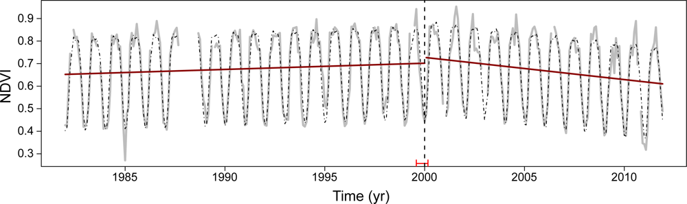
If there are gaps in the time series y_t, these observations can simply be omitted prior to estimation of the model parameters. These parameters can still be identified consistently, unless all observations at certain frequencies are missing. In this way, the quality flags could be used to omit unreliable observations (see example in Figure 1). The season-trend model takes the underlying trend and seasonal variation within a time series into account so that season-trend patterns are removed in the resulting residuals. This corresponds to approaches where in multiple steps a time series is “detrended” and “deseasonalized” (e.g., [5]), whereas here the adjustment was performed in a single step by OLS fitting of the season-trend model. If no trend and/or no seasonality are present in the data investigated, the corresponding elements of the regressor can also be omitted. The proposed season-trend model is analogous to the BFAST [16] approach, but differs in a way that it has been optimized for detecting the most influential trend shift in the time series, as opposed to multiple smaller shifts. Also, BFAST iteratively fits a separate seasonal and trend model and is therefore computationally more intensive. Figure 1 illustrates a season-trend model (dashed black line) fitted to an NDVI time series (gray) while accounting for the most influential trend shift.

Based on the season-trend model introduced above, we assessed whether the temporal trend was a linearly developing equilibrium or included shifts, i.e., if the model parameters remained stable or were changing over time. In statistical and econometric literature, this approach is known as testing for structural changes. Structural, in this context, refers to the statistical property of the time series and not to characteristics of a vegetation canopy. A broad range of statistical tests for structural change detection have been suggested, using linear regression models in particular [26–28]. Because the season-trend model can be formulated as an OLS linear regression, all of these methods can be leveraged directly. Below, we focus on structural change tests based on moving sums (MOSUMs) of OLS residuals [29] that have higher power for detecting changes in the trend (i.e., the parameters α₁ and α₂) while being less sensitive to changes in cyclical patterns [30], i.e., to phenological changes. Given detection of a significant structural change, the associated breakpoint was estimated [31]. This is referred to as dating of the breakpoint. Both testing and dating were carried out using the implementation of [32,33] in the R software for statistical computing [34].

The mentioned MOSUM test for break detection is based on moving sums with bandwidth h of the OLS residuals ɛ̂_t (Equation (2)). The bandwidth h operates as a smoothing parameter, although only for the break detection on OLS residuals and not for the subsequent breakpoint estimation on the NDVI3g time series.

$$M_t=\frac{1}{\widehat{\sigma }\sqrt{n}}\sum _{s=t-h+1}^t{\widehat{\varepsilon }}_s$$

(2)

where h = 40 for our application (see below for more details). If the model remains stable, the MOSUM process M_t should be close to zero and fluctuate only randomly. However, if a structural change occurs, M_t will deviate systematically from zero. A structural break was declared if the maximum absolute value max_t|M_t| exceeded its 5% asymptotic critical value [29].

If the MOSUM test signaled a significant instability in the season-trend model (at 5% level), we captured this change by estimating one breakpoint and fitting separate season-trend models to the two segments before and after the break. The breakpoint was estimated (or dated) using OLS, i.e., by minimizing the combined sum of squared residuals from the two segments. Confidence intervals for the breakpoint estimates can also be calculated [31]. To ensure that the 8 regression parameters (2 trend and 6 season parameters) of the season-trend model can be sensibly estimated in both segments, a minimal segment size of 40 observations (i.e., 3.5 years) was enforced and the MOSUM bandwidth was chosen correspondingly.

Although such a two-segment season-trend model may still contain further structural changes, its breakpoint consistently identifies the largest shift (in terms of the residual sum of squares), see [35].

In summary, this modeling approach either identifies no break at all (if the MOSUM test results is non-significant) or a single “most important” break that can occur between 1985 and 2008. Typically, if such a break is found, it can be interpreted as a long-term change. However, breakpoints occurring very early or late in the sampling period need to be carefully interpreted with respect to their long-term significance, since one of the two segments might reflect a short-lived process.

2.3. Ecological Characterization of Trend Shifts

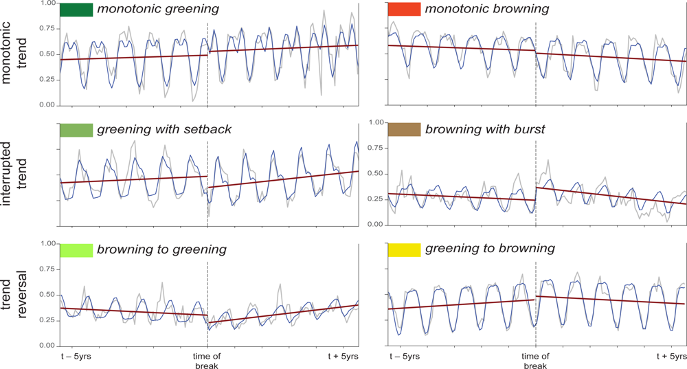
After having detected a trend shift within the time series, a main challenge is interpreting the changes. One approach is the characterization of the shifts into classes, which are expected to have different driving processes and ecological implications. Six major classes (referred to as trend types) are therefore defined as follows: two classes for monotonic change (increasing or decreasing), two for interrupted trends and two for trend reversals (greening to browning or vice versa). In Figure 2, these are represented by the three rows (top to bottom), while the columns separate recent greening from recent browning. In addition to these trend types, individual segments may be stable (i.e., in steady-state equilibrium), meaning that no substantial change was detected during the corresponding period. A threshold of 0.25%/year was used, below which trends were regarded to be stable. Cases with stable segments are not shown but automatically imply monotonic change in the other segment.

Each of the trend types can be induced by a wide range of underlying processes and likely by a combination of more than one process. Some types, however, can be attributed to certain processes with higher likeliness than others. For example, in our case of long observation periods (i.e., 30 years), monotonic changes are likely induced by changes in growth-limiting climatologies [3], although persistent land-use change (e.g., forest-crop conversion and urbanization) may also be considered as a candidate driver [36]. In water-limited environments, an abrupt increase in vegetation activity (or burst), followed by a gradual decrease, may indicate response of vegetation to a relatively wet period. The wet period may, for instance, be induced by oceanic oscillations, like the El Nino/La Nina Southern Oscillation (ENSO). In higher northern latitudes, the same type of trend change is more likely a result of few anomalous warm years with less snow-covered days. An abrupt negative change (or setback), on the other hand, may be attributable to human interventions (e.g., logging followed by regrowth). Natural drivers, in such cases, may be wildfire or diseases followed by a period of gradual recovery. These examples include short-lived events to cause a burst or setback in the gradual trend. From a global change perspective, the cases where gradual trends reverse may be most interesting. This type of sustained trend changes may indicate major shifts between greening and browning regimes. Such shifts were suggested in literature [9], but also debated [10,11].

Apart from these biophysical candidates, trends shifts may have been induced by data artifacts, including differences between AVHRR-2 and AVHRR-3 or by NOAA platform changes [14,37]. However, we did not find a relationship with AVHRR sensor changes and there is a sound basis to assume that such events have been effectively corrected [20,38].

3. Results and Discussion

3.1. Spatial and Temporal Distribution of Trend Breaks

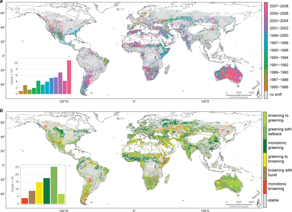
All but the monotonic trend types are characterized by a break at a certain point in time. By assessing the timing of the breakpoints, we found an increasing number of events occurring in more recent times (Figure 3(a), inset). With few exceptions, the increase appeared monotonic and almost linear, especially until the 2000s. This suggests that the relatively stable vegetation regimes of the early periods of the GIMMS time span have changed to higher turnover rates. This, in turn, supports the premise that monotonic trends do not suffice to capture the change in many parts of the world and that shifts in vegetation activity trends should therefore not be ignored.

Early shifts (1980s) were concentrated in Botswana, Northeast Brazil and some parts of Europe (Figure 3(a), orange and light green hues). Later dates appeared geographically less confined, but showed distinct regional patterns in most cases. Several of these patterns are discussed in the next section. The better part of the latest shifts (after 2005) were concentrated in Australia and Argentina and coincided with a green-up reversal (see Section 3.2.3). In a framework of long-term structural shifts, careful interpretation of these early and late shifts is required. In such cases, one of the gradual-change segments is short, which puts (recovery from) short-term disturbances, rather than long-term shifts, forward as candidate driver.

At global scale, the 1992 Mt Pinatubo eruption was found to have affected vegetation activity [39], but we did not find firm indications for a structural shift in our results. The years after the event show a slightly higher representation of breakpoints, but it would be premature to conclude on a causative relationship. Likely, the eruption lead to disturbances from which vegetation systems have recovered on a shorter time scale than addressed in this study.

3.2. Geographical Patterns of Trend Types

Following Figure 2, six trend types were considered. A global count of grid cells (Figure 3(b), inset) indicated that greening trends (green hues) prevailed, which is in line with conclusions of previous studies [2,3,12,13], although most of these trends seem to have experienced a setback. At the same time, many of the grid cells with a browning trend contained a burst in which canopies showed anomalously high chlorophyll absorption, possibly because of a short-term relaxation of climatic growth constraints. Another substantial part of the browning trends recently changed into greening (e.g., parts of Australia and Argentina in the late 2000s). As a consequence, monotonic browning represents the smallest class. We assessed the possibility of two stable segments separated by an abrupt change event, but too few examples of this type were found to include them in a separate class.

Each of the trend types occurred in various geographical regions (Figure 3(b), map). The geographical distribution of the three main trend categories (rows in Figure 2) is discussed in the following sections. These sections point out some of the most conspicuous regions and are not intended to be an exhaustive discussion on candidate drivers. A discussion on potential relationships between NDVI trends and various drivers is, among others, provided by Fensholt et al.[40].

3.2.1. Monotonic Change

A wide range of studies previously quantified monotonic NDVI changes in specific regions, or globally. For illustration and comparison, Figure 4 shows the magnitude of monotonic change (1982–2006). Figure 3(b) confirms that vegetation activity in certain regions showed a monotonic behavior, even if trend shifts are accounted for. Examples include the northern Great Plains, parts of eastern Europe and eastern China. In other regions, however, the assumption of monotonicity (Figure 4) may have overlooked a possible interruption (e.g., western India and Asia Minor) or may have averaged out separate periods with significant change, resulting in unjust classification of the region as stable (e.g., southern Argentina, northern Kazakstan).

Conspicuous greening was found in large parts of the Northern Hemisphere during the last decades of the previous century [2]. With a 12 year longer dataset, indications for this phenomenon are still present. Parts of Europe and Asia—mainly between 40 and 60 degrees latitude—show signs of a continuous increase in vegetation activity, without significant interruptions. The northern part of the Great Plains formed the largest region with monotonic greening in the Americas. It is beyond the capacity of this study to interpret driving processes, but literature suggests that an increase in precipitation boosted crop yields in these regions [41]. Similarly, large crop-land areas in eastern China (e.g., Shandong province) and in the Indo-Gangetic Plain showed monotonic increase in vegetation activity.

The tundra and boreal forests were largely excluded from our analysis, based on GIMMS quality flags (i.e., long snow cover). These regions, however, were previously found to be least affected by discontinuities in vegetation activity trends [8]. Under warming conditions, monotonic greening has been reported in tundra regions, while boreal forests showed signs of (late-summer) browning, possibly drought-induced [42]. Recently, these patterns seem to have amplified rather than reversed [43].

Extensive monotonic green-up was furthermore found in a latitudinal belt south of the Sahel, roughly in the sub-humid zone around 5°N. This coincides with the southern part of the documented “Sahelian green-up” [44–46] and covers (parts of) Nigeria, Togo, Ghana, among other countries. The semi-arid Sahel itself rather showed an early-2000s reversal towards reduced vegetation activity after two decades of prosperous growth. In the northern and driest parts of the Sahel, in turn, the greening pattern persisted, despite a setback around the same time.

A monotonic decrease in vegetation activity appeared to have sustained in substantially fewer regions. Few examples include the border region between Paraguay and Bolivia and some hotspots in northern China (Heilongjiang province). Most of the browning trends, however, were interrupted by a burst in vegetation activity.

3.2.2. Interrupted Gradual Change

Interrupted greening was the most common class in our results and interrupted browning appeared also more common than monotonic browning (Figure 3(b), inset). The types of shifts showed different temporal distributions (Figure 5), with bursts concentrated in the 1990s and setbacks or browning reversals just after the millennium transition. However, regional variations in this temporal pattern exist. A setback around 1990 was for instance found in eastern Brazil after which the region showed a continuous increase again. This increase was not picked up by the previous monotonic analysis (Figure 4). Discontinuities around 2000 were found in southeastern United States and in the countries in southern Africa. Noticeably, Botswana appeared as greening hotspot in the monotonic analysis while this pattern seemed more complicated with trend shifts included. The trends changed in the late 1980s, when the central part of Botswana experienced a burst. The gradual change afterwards, however, was found to be negative rather than positive.

A region with similar patterns is the Horn of Africa. Parts were previously found to become greener, but Figure 3(b) suggests that this signal might be attributable to a short-term burst in the 1990s (Ethiopia early 1990s, Somalia and Kenya late 1990s). The gradual change appeared either negative throughout the full period or reversed into a negative trend. The resulting decline in vegetation activity seems to have amplified recently due to a period of persistently poor rains, causing severe food insecurity in the region [18,47].

3.2.3. Trend Reversals

As mentioned before, there is a well documented agreement on a net greening pattern since the early 1980s, especially in the Northern Hemisphere [2,13]. It has, however, also been suggested (and debated) that vegetation activity peaked around the millennium transition, after which browning trends took over, most notably in the Southern Hemisphere [8,9]. For the majority of the trend reversals detected in this study, greening turned into browning (Figure 3(b), inset), which substantiates the hypothesized reduction in vegetation activity. The timing of these reversals, for the better part, coincides with the late 1990s and early 2000s (Figure 5). Substantially fewer regions with reversals into greening were found and most of these were confined to the latest years of the GIMMS time span. Therefore, they may represent a short-lived process. In terms of number of grid cells, the area under browning trends increased from ca. 20 × 10⁴ to ca. 28 × 10⁴, which is equivalent to an increase of 40%.

The greening-to-browning reversals appeared geographically diverse, but prominent regions include parts of Western Australia, the Sahel, Argentina, northern Kazakhstan and the Middle East. In these regions, a monotonicity-assumption may cause reversed trend segments to average out, resulting in a stable qualification or a relatively low net change. Indications for this effect were, for instance, found in Australia. Greening was previously found in Western Australia and browning in the central parts of Australia, while the eastern regions appeared stable (Figure 4). According to Figure 3(b), however, large parts of the central and eastern regions have experienced a recent green-up reversal while a greening-to-browning hotspot was found in Western Australia. The green-up can likely be attributed to the recent rainfall in eastern Australia [48], which boosted vegetation activity. The western browning reversal occurred earlier, i.e., around the millennium transition, and may be attributable to droughts [9,48,49]. Similar reversals were found in a latitudinal band in central Asia, with a longitudinal gradient in the timing (late 1980s in the West up to late 1990s in the East).

In the Sahel, similar reversals were found before the time span of satellite records, coinciding with the onset of a long-term drought around 1969 [50]. An alternation between two land cover states, a “wet Sahel” and a “dry Sahel”, each of which may persist for decades at a time, has been suggested by Foley et al.[50]. Shifts between the two states are preceded and induced by gradual processes like land degradation and sea-surface temperature. In large parts of Africa, oceanic oscillations are likely to play a role in these vegetation dynamics [51].

3.3. Contribution to Global Change Studies and Outlook

This study extends results identified by previous studies. First, compared with studies that exclusively targeted monotonic trends [12,13], the presented approach provides a more sophisticated insight in the way vegetation activity varied during the past decades. The accuracy of previous magnitude estimates is not debated, but the pathway to arrive at the considered magnitude appeared non-monotonic for 74% of the grid cells with trends. This, in combination with the increased turnover rate, implies that the complexity of biosphere alterations and responses to various external forces has increased. This should be addressed in more detail by studying randomness in the occurrence of trend shifts, since an increase would indicate accelerated changes in vegetation processes. Accounting for trend shifts, while analyzing GIMMS or equivalent time series, provides a better representation of multi-decadal biosphere dynamics and the drivers of alteration herein. The main challenge is to incorporate these dynamics in models that provide physical links with human and climatic drivers. Many factors prevent this from being a straightforward exercise, including lag effects in the response of ecosystems, multi-actor systems with mutual influences and also the nature of broadband indices like NDVI, which aggregate a multitude of effects into a single metric. Second, the observed dynamics may provide a means to compare against modeled biosphere dynamics [3,9]. At global scale and long temporal scales, field validation of both types of products is not feasible, calling for careful interpretation. This previously resulted in a debate about the sensitivity of applied models to certain parameters, notably temperature [10,11]. The current study is based on observations and revealed actual dynamics recorded by satellites, which, with the benefit of hindsight, may serve to verify model simulations. The current study investigated type and timing of trend shifts; further work should investigate the associated changes in the rate of gradual change induced by these trend shifts.

4. Conclusions

The demonstrated approach for the detection and classification of shifts in vegetation activity trends is the first to consistently assess different types of changes on the biosphere during the past decades. The availability of third generation 1982–2011 Global Inventory Modeling and Mapping Studies (GIMMS) data was crucial for this study. The analysis provided new insights to several aspects of global vegetation dynamics:

• Monotonicity was found for 26 percent of the analyzed 0.083° grid cells with a significant temporal trend. Shifts in vegetation activity trends were found for the remaining land surface: either an interruption (greening with “setback”, respectively browning with “burst”) or a reversal (greening-to-browning or v.v.). Setbacks were found in many greening trends, in particular in western India, Asia Minor and Western Australia. Bursts in browning trends were conspicuous in the Horn of Africa and in northern Patagonia (Rio Negro province).

• Over time, an increase in the frequency of trend shifts was found. With respect to the 1980s, a four times larger area with changing trends was found in the 2000s. This suggests that relatively stable vegetation regimes have changed towards higher turnover rates, implying an increase in the complexity of biospheric alterations and responses to external forces.

• Greening trends were found to have reversed into browning more than the other way around, which indicates a decline in vegetation activity. Compared with the 1980s, negative vegetation activity trends were found to have increased in area about 40% over time. Most of the greening-to-browning reversals occurred around the millennium transition. They were not confined to a single geographical region, but extended across all continents. Notable regions include parts of southern Argentina, northern Kazakhstan, the Middle East, the Sahel, Eastern Africa and Western Australia. The other way around, browning-to-greening reversals were found in central Australia and northern Argentina. These mainly occurred in recent times (late 2000s) and may therefore represent short-lived processes.

Further analysis is needed to attribute observed trend changes to cause-effect relationships, as well as validating these trend changes using evidence from climatic, economic, and other human impact data alike.

References

- Gutman, G.; Ignatov, A. Global land monitoring from AVHRR: Potential and limitations. Int. J. Remote Sens 1995, 16, 2301–2309. [Google Scholar]
- Zhou, L.; Tucker, C.J.; Kaufmann, R.K.; Slayback, D.A.; Shabanov, N.V.; Myneni, R.B. Variations in northern vegetation activity inferred from satellite data of vegetation index during 1981 to 1999. J. Geophys. Res 2001, 106, 20269–20283. [Google Scholar]
- Nemani, R.R.; Keeling, C.D.; Hashimoto, H.; Jolly, W.M.; Piper, S.C.; Tucker, C.J.; Myneni, R.B.; Running, S.W. Climate-driven increases in global terrestrial net primary production from 1982 to 1999. Science 2003, 300, 1560–1563. [Google Scholar]
- De Jong, R.; de Bruin, S.; Schaepman, M.E.; Dent, D.L. Quantitative mapping of global land degradation using earth observations. Int. J. Remote Sens 2011, 32, 6823–6853. [Google Scholar]
- Potter, C.; Tan, P.N.; Steinbach, M.; Klooster, S.; Kumar, V.; Myneni, R.; Genovese, V. Major disturbance events in terrestrial ecosystems detected using global satellite data sets. Glob. Change Biol 2003, 9, 1005–1021. [Google Scholar]
- Slayback, D.A.; Pinzon, J.E.; Los, S.O.; Tucker, C.J. Northern hemisphere photosynthetic trends 1982–99. Glob. Change Biol 2003, 9, 1–15. [Google Scholar]
- Angert, A.; Biraud, S.; Bonfils, C.; Henning, C.C.; Buermann, W.; Pinzon, J.; Tucker, C.J.; Fung, I. Drier summers cancel out the CO2 uptake enhancement induced by warmer springs. Proc. Natl. Acad. Sci. USA 2005, 102, 10823–10827. [Google Scholar]
- De Jong, R.; Verbesselt, J.; Schaepman, M.E.; de Bruin, S. Trend changes in global greening and browning: Contribution of short-term trends to longer-term change. Glob. Change Biol 2012, 18, 642–655. [Google Scholar]
- Zhao, M.; Running, S.W. Drought-induced reduction in global terrestrial net primary production from 2000 through 2009. Science 2010, 329, 940–943. [Google Scholar]
- Samanta, A.; Costa, M.H.; Nunes, E.L.; Vieira, S.A.; Xu, L.; Myneni, R.B. Comment on “drought-induced reduction in global terrestrial net primary production from 2000 through 2009”. Science 2011, 333, 1093. [Google Scholar] [CrossRef]
- Medlyn, B.E. Comment on “drought-induced reduction in global terrestrial net primary production from 2000 through 2009”. Science 2011, 333, 1093. [Google Scholar] [CrossRef]
- De Jong, R.; de Bruin, S.; de Wit, A.; Schaepman, M.E.; Dent, D.L. Analysis of monotonic greening and browning trends from global NDVI time-series. Remote Sens. Environ 2011, 115, 692–702. [Google Scholar]
- Bai, Z.G.; Dent, D.L.; Olsson, L.; Schaepman, M.E. Proxy global assessment of land degradation. Soil Use Manage 2008, 24, 223–234. [Google Scholar]
- De Beurs, K.M.; Henebry, G.M. A statistical framework for the analysis of long image time series. Int. J. Remote Sens 2005, 26, 1551–1573. [Google Scholar]
- Julien, Y.; Sobrino, J.A. Global land surface phenology trends from GIMMS database. Int. J. Remote Sens 2009, 30, 3495–3513. [Google Scholar]
- Verbesselt, J.; Hyndman, R.; Newnham, G.; Culvenor, D. Detecting trend and seasonal changes in satellite image time series. Remote Sens. Environ 2010, 114, 106–115. [Google Scholar]
- Verbesselt, J.; Hyndman, R.; Zeileis, A.; Culvenor, D. Phenological change detection while accounting for abrupt and gradual trends in satellite image time series. Remote Sens. Environ 2010, 114, 2970–2980. [Google Scholar]
- Verbesselt, J.; Zeileis, A.; Herold, M. Near real-time disturbance detection using satellite image time series. Remote Sens. Environ 2012, 123, 98–108. [Google Scholar]
- Schimel, D.S.; House, J.I.; Hibbard, K.A.; Bousquet, P.; Ciais, P.; Peylin, P.; Braswell, B.H.; Apps, M.J.; Baker, D.; Bondeau, A.; et al. Recent patterns and mechanisms of carbon exchange by terrestrial ecosystems. Nature 2001, 414, 169–172. [Google Scholar]
- Tucker, C.; Pinzon, J.; Brown, M.; Slayback, D.; Pak, E.; Mahoney, R.; Vermote, E.; El Saleous, N. An extended AVHRR 8 km NDVI dataset compatible with MODIS and SPOT vegetation NDVI data. Int. J. Remote Sens 2005, 26, 4485–4498. [Google Scholar]
- Tucker, C.J. Red and photographic infrared linear combinations for monitoring vegetation. Remote Sens. Environ 1979, 8, 127–150. [Google Scholar]
- Holben, B.N. Characteristics of maximum-value composite images from temporal AVHRR data. Int. J. Remote Sens 1986, 7, 1417–1434. [Google Scholar]
- Geerken, R.A. An algorithm to classify and monitor seasonal variations in vegetation phenologies and their inter-annual change. ISPRS J. Photogramm 2009, 64, 422–431. [Google Scholar]
- Julien, Y.; Sobrino, J.A. Comparison of cloud-reconstruction methods for time series of composite NDVI data. Remote Sens. Environ 2010, 114, 618–625. [Google Scholar]
- Cryer, J.D.; Chan, K.S. Time Series Analysis–With Applications in R, 2nd ed; Springer-Verlag: New York, NY, USA, 2008. [Google Scholar]
- Andrews, D.W.K. Tests for parameter instability and structural change with unknown change point. Econometrica 1993, 61, 821–856. [Google Scholar]
- Kuan, C.M.; Hornik, K. The generalized fluctuation test: A unifying view. Econom. Rev 1995, 14, 135–161. [Google Scholar]
- Zeileis, A. A unified approach to structural change tests based on ML scores, F statistics, and OLS residuals. Econom. Rev 2005, 24, 445–466. [Google Scholar]
- Chu, C.S.J.; Hornik, K.; Kuan, C.M. MOSUM tests for parameter constancy. Biometrika 1995, 82, 603–617. [Google Scholar]
- Ploberger, W.; Krämer, W. The CUSUM test with OLS residuals. Econometrica 1992, 60, 271–285. [Google Scholar]
- Bai, J.; Perron, P. Computation and analysis of multiple structural change models. J. Appl. Econom 2003, 18, 1–22. [Google Scholar]
- Zeileis, A.; Leisch, F.; Hornik, K.; Kleiber, C. Strucchange: An R package for testing for structural change in linear regression models. J. Stat. Softw 2002, 7, 1–38. [Google Scholar]
- Zeileis, A.; Kleiber, C.; Krämer, W.; Hornik, K. Testing and dating of structural changes in practice. Comput. Stat. Data Anal 2003, 44, 109–123. [Google Scholar]
- R Development Core Team. R: A Language and Environment for Statistical Computing; R Foundation for Statistical Computing: Vienna, Austria, 2012. [Google Scholar]
- Chong, T.T.L. Partial parameter consistency in a misspecified structural change model. Econom. Lett 1995, 49, 351–357. [Google Scholar]
- Ramankutty, N.; Graumlich, L.; Achard, F.; Alves, D.; Chhabra, A.; DeFries, R.; Foley, J.A.; Geist, H.J.; Houghton, R.A.; Klein Goldewijk, K.; et al. Global Land-Cover Change: Recent Progress, Remaining Challenges. In Land-Use and Land-Cover Change: Local Processes and Global Impacts; Lambin, E.F., Geist, H.J., Eds.; Springer-Verlag: Berlin, Germany, 2006; pp. 9–39. [Google Scholar]
- Latifovic, R.; Pouliot, D.; Dillabaugh, C. Identification and correction of systematic error in NOAA AVHRR long-term satellite data record. Remote Sens. Environ 2012, 127, 84–97. [Google Scholar]
- Kaufmann, R.K.; Zhou, L.; Knyazikhin, Y.; Shabanov, V.; Myneni, R.B.; Tucker, C.J. Effect of orbital drift and sensor changes on the time series of AVHRR vegetation index data. IEEE Trans. Geosci. Remote Sens 2000, 38, 2584–2597. [Google Scholar]
- Lucht, W.; Prentice, I.C.; Myneni, R.B.; Sitch, S.; Friedlingstein, P.; Cramer, W.; Bousquet, P.; Buermann, W.; Smith, B. Climatic control of the high-latitude vegetation greening trend and Pinatubo effect. Science 2002, 296, 1687–1689. [Google Scholar]
- Fensholt, R.; Langanke, T.; Rasmussen, K.; Reenberg, A.; Prince, S.D.; Tucker, C.; Scholes, R.J.; Le, Q.B.; Bondeau, A.; Eastman, R.; et al. Greenness in semi-arid areas across the globe 1981–2007—An Earth observing satellite based analysis of trends and drivers. Remote Sens. Environ 2012, 121, 144–158. [Google Scholar]
- Neigh, C.S.R.; Tucker, C.J.; Townshend, J.R.G. North American vegetation dynamics observed with multi-resolution satellite data. Remote Sens. Environ 2008, 112, 1749–1772. [Google Scholar]
- Goetz, S.J.; Epstein, H.E.; Bhatt, U.S.; Jia, G.J.; Kaplan, J.O.; Lischke, H.; Yu, Q.; Bunn, A.G.; Lloyd, A.H.; Alcaraz-Segura, D.; et al. Recent Changes in Arctic Vegetation: Satellite Observations and Simulation Model Predictions. In Eurasian Arctic Land Cover and Land Use in a Changing Climate; Gutman, G., Reissell, A., Eds.; Springer-Verlag: Amsterdam, The Netherlands, 2011; pp. 9–36. [Google Scholar]
- Beck, P.S.A.; Goetz, S.J. Satellite observations of high northern latitude vegetation productivity changes between 1982 and 2008: Ecological variability and regional differences. Environ. Res. Lett. 2011. [Google Scholar] [CrossRef]
- Hickler, T.; Eklundh, L.; Seaquist, J.W.; Smith, B.; Ardö, J.; Olsson, L.; Sykes, M.T.; Sjöström, M. Precipitation controls Sahel greening trend. Geophys. Res. Lett 2005, 32, 2–5. [Google Scholar]
- Anyamba, A.; Tucker, C.J. Analysis of Sahelian vegetation dynamics using NOAA-AVHRR NDVI data from 1981–2003. J. Arid Environ 2005, 63, 596–614. [Google Scholar]
- Olsson, L.; Eklundh, L.; Ardö, J. A recent greening of the Sahel–trends, patterns and potential causes. J. Arid Environ 2005, 63, 556–566. [Google Scholar]
- Funk, C. We thought trouble was coming. Nature 2011. [Google Scholar] [CrossRef]
- McGrath, G.S.; Sadler, R.; Fleming, K.; Tregoning, P.; Hinz, C.; Veneklaas, E.J. Tropical cyclones and the ecohydrology of Australia’s recent continental-scale drought. Geophys. Res. Lett. 2012. [Google Scholar] [CrossRef]
- Donohue, R.J.; McVICAR, T.R.; Roderick, M.L. Climate-related trends in Australian vegetation cover as inferred from satellite observations, 1981–2006. Glob. Change Biol 2009, 15, 1025–1039. [Google Scholar]
- Foley, J.A.; Coe, M.T.; Scheffer, M.; Wang, G. Regime shifts in the sahara and sahel: Interactions between ecological and climatic systems in Northern Africa. Ecosystems 2003, 6, 524–532. [Google Scholar]
- Brown, M.E.; de Beurs, K.; Vrieling, A. The response of African land surface phenology to large scale climate oscillations. Remote Sens. Environ 2010, 114, 2286–2296. [Google Scholar]
Share and Cite
De Jong, R.; Verbesselt, J.; Zeileis, A.; Schaepman, M.E. Shifts in Global Vegetation Activity Trends. Remote Sens. 2013, 5, 1117-1133. https://doi.org/10.3390/rs5031117
De Jong R, Verbesselt J, Zeileis A, Schaepman ME. Shifts in Global Vegetation Activity Trends. Remote Sensing. 2013; 5(3):1117-1133. https://doi.org/10.3390/rs5031117
Chicago/Turabian StyleDe Jong, Rogier, Jan Verbesselt, Achim Zeileis, and Michael E. Schaepman. 2013. "Shifts in Global Vegetation Activity Trends" Remote Sensing 5, no. 3: 1117-1133. https://doi.org/10.3390/rs5031117