1. Introduction
The application of genome-wide association (GWA) studies has become increasingly common, due to the availability of genome-wide dense marker maps at relatively low-cost. GWA studies typically can have two main objectives. The first objective is to derive the position of a gene or a genomic region that has an influence on one or more traits of interest. Common examples are identification of disease loci in human (Thomson, Reference Thomson1995), or identification of quantitative trait loci (QTLs) in livestock (Weller et al., Reference Weller, Kashi and Soller1990; Andersson & Georges, Reference Andersson and Georges2004). The second objective of GWA is to predict the genetic potential or phenotype of an individual for a certain trait. Examples are estimation of breeding values in livestock to enable genomic selection (Meuwissen et al., Reference Meuwissen, Hayes and Goddard2001), or prediction of the (genetic) susceptibility of an individual for a disorder or disease (Wray et al., Reference Wray, Goddard and Visscher2007). Generally, the applied models for both types of GWA studies may be the same, although fine-tuning for one of both objectives may result in subtle differences in the applied models (Calus et al., Reference Calus, Meuwissen, Windig, Knol, Schrooten, Vereijken and Veerkamp2009).
GWA studies are typically performed using markers such as single nucleotide polymorphisms (SNPs) that represent a sample of the variation in the genome. Another source of structural genomic variation is in the form of differences between different individuals in numbers of copies of genomic regions, referred to as copy number variation (CNV) or copy number polymorphisms (CNPs). Recent studies in human genetics have revealed that CNV may underlie an appreciable amount of variation at the trait level (Khaja et al., Reference Khaja, Zhang, MacDonald, He, Joseph-George, Wei, Rafiq, Qian, Shago, Pantano, Aburatani, Jones, Redon, Hurles, Armengol, Estivill, Mural, Lee, Scherer and Feuk2006; Locke et al., Reference Locke, Sharp, McCarroll, McGrath, Newman, Cheng, Schwartz, Albertson, Pinkel, Altshuler and Eichler2006). Moreover, it has been shown that CNVs can be associated with disease susceptibility and that disease genes are located in CNV regions (Sebat et al., Reference Sebat, Lakshmi, Troge, Alexander, Young, Lundin, Maner, Massa, Walker, Chi, Navin, Lucito, Healy, Hicks, Ye, Reiner, Gilliam, Trask, Patterson, Zetterberg and Wigler2004; Blasko et al., Reference Blasko, Szeplaki, Varga, Ronai, Prohaszka, Sasvari-Szekely, Visy, Farkas and Fust2007; Kehrer-Sawatzki, Reference Kehrer-Sawatzki2007; Zhang et al., Reference Zhang, Gu, Hurles and Lupski2009). GWA studies typically use dense SNP maps to associate genetic variation with genomic regions. Considering that CNPs may be directly associated with phenotypic variation, an important question is whether this phenotypic variance can also be captured using a dense SNP map, or whether CNPs should be genotyped and included in GWA studies. In the situation where CNPs and SNPs are located in the same regions and therefore physically closely related, the difference in mutation rates and number of alleles between the two types of loci may still result in relatively low linkage disequilibrium (LD) between both types of loci. Genotyping of CNP loci may be straightforward for loci with only two alleles, each representing a different number of segregating copies, but may be difficult for loci with more than two segregating alleles (Locke et al., Reference Locke, Sharp, McCarroll, McGrath, Newman, Cheng, Schwartz, Albertson, Pinkel, Altshuler and Eichler2006). A proposed solution to this problem is to use raw (continuous) hybridization intensities at those CNP loci, rather than derived (discrete) genotypes to provide an estimate of the number of copies (over both gametes) in an individual (Locke et al., Reference Locke, Sharp, McCarroll, McGrath, Newman, Cheng, Schwartz, Albertson, Pinkel, Altshuler and Eichler2006). In addition to measuring the CNP genotypes for all individuals, they may be predicted for some individuals. The predicted number of copies (over both gametes) could also be used as a continuous measure of the CNP locus.
The objective of this study was to investigate, both empirically and deterministically, the ability to explain genetic variation resulting from a CNP by including the CNP, either by its genotype or by a continuous derivation thereof, alone or together with a nearby SNP in the model.
2. Material and methods
Formulae are derived to predict the captured variance at CNP loci when CNP genotypes are not measured with 100% accuracy. Predictions from those formulae are compared to R 2 values from simulated data. To derive reasonable distributions of LD between SNP and CNP loci, data were simulated with two segregating CNP and several segregating SNP loci. The derived distributions were used to gain insight into the LD between SNP and CNP loci, and to inform additional simulations to investigate the possibility to associate genetic variance caused by a CNP locus with allelic variation of a linked SNP. Additionally, the benefit of including CNP phenotypes, i.e. a continuous measure or prediction for CNP genotypes, or CNP genotypes in the model was investigated.
(i) Simulations to estimate associations between segregating SNP and CNP loci
An important characteristic that we want to derive is the association between CNP and SNP loci. A measure of the association between a biallelic (SNP) locus and a multiallelic locus (in this case a CNP), was presented by Zhao et al. (Reference Zhang, Nettleton, Soller and Dekkers2005) as
where Ai is one of k alleles at the multiallelic (CNP) locus and Q is one of the two alleles at the biallelic (SNP) locus. Considering this formula, the association between an SNP and a CNP locus depends on the number of alleles at the CNP locus, the allele frequencies at the SNP and CNP loci, and the frequencies of haplotypes consisting of CNP and SNP alleles. These parameters, in turn, depend on the population history and the mutation rates at both loci. Therefore, simulation of a large number of replicated datasets will give insight into the distribution of r 2 values between SNP and CNP loci, for the simulated population history and mutation rates.
To derive the distribution of LD between an SNP and a CNP, d cM apart, we simulated a population with 500 individuals that were randomly mated for 4000 generations. Twenty CNP loci were simulated on the same position and 70 SNP loci; 10 SNPs at each of seven positions located at 0·0, 0·0, 0·01, 0·1, 0·5, 1·0 and 2·0 cM distance of the CNP loci (Fig. 1). Two sets of SNPs were simulated at a distance of 0·0 to allow estimation of SNP–SNP LD at 0·0 cM distance. All CNP and SNP loci had alleles 1 and 2 segregating in the first generation, where both alleles were drawn per individual and locus with equal chance. Segregating loci in the first generation combined with 4000 generations of random mating ensure reaching a mutation-drift balance. The applied mutation rate for the SNP loci was 2×10⁻⁸ per haploid locus per generation (e.g. Drake et al., Reference Drake, Charlesworth, Charlesworth and Crow1998; Kumar & Subramanian, Reference Kumar and Subramanian2002). Initially, SNP alleles were coded as 1 or 2. A mutation on an SNP locus changed an allele 1 (2) to become 2 (1). The applied mutation rate for the CNP loci was 10−4 per haploid locus per generation based on several reported estimates (Tusieluna & White, Reference Tusieluna and White1995; Nuzhdin, Reference Nuzhdin1999; Shaffer & Lupski, Reference Shaffer and Lupski2000; van Ommen, Reference van Ommen2005; Repping et al., Reference Repping, van Daalen, Brown, Korver, Lange, Marszalek, Pyntikova, van der Veen, Skaletsky, Page and Rozen2006). For 10 CNP loci, it was assumed that a mutation event caused the number of copies to decrease or increase by one copy with equal probability. Whenever a mutation occurred at a locus with 0 copies, the only possible outcome was 1 copy. These CNPs are from here on referred to as CNPm loci. For the other 10 CNPs, as well as for the SNP loci, a mutation of allele 1 always resulted in allele 2, and a mutation of allele 2 always resulted in allele 1. This latter type of CNP therefore represented an SNP with the assumed mutation rate of a CNP. These CNPs are from here on referred to as CNP2. Recombination, based on Haldane's mapping function, was considered among all loci.

Fig. 1. The simulated marker map, with one CNP locus with only 2 alleles (CNP2), one CNP locus with two or more alleles (CNPm), and SNP loci at respectively 0·0, 0·1, 0·5, 1·0 and 2·0 cM distance with 10 SNPs at each locus.
In total, 100 000 replicates were simulated. From those replicates, distributions for allele frequencies at SNP and CNP loci, r 2 values between SNP and CNP loci, and the number of alleles at CNP loci, were derived for each of the six considered distances, using the simulated genotypes from the last generation (i.e. using 500 individuals).
(ii) Simulation of phenotypes with a CNP and an SNP
The first set of simulations yielded a large number of haplotypes combining alleles from an SNP locus and a CNP locus. The obtained distributions of the frequencies of those haplotypes, in which a CNPm locus was included, were used to simulate six sets of data with one segregating SNP and one segregating CNP locus, again with different distances (0·0, 0·01, 0·1, 0·5, 1·0 and 2·0 cM) between those loci. Those simulated datasets in turn were used to evaluate the accuracy and bias of models including different combinations of SNP and CNP information (as explained in the next section). Each simulated dataset contained 500 individuals. Each individual received haplotypes, i.e. combinations of SNP and CNP alleles, with probabilities equal to the haplotype frequencies from the previous simulations. This ensured that this simulation represented the original simulated population. Each CNP allele received an effect on the phenotype of the individuals such that the CNP locus explained 10% of the total phenotypic variance. The remaining 90% of the phenotypic variation was explained by a residual effect, drawn for each individual from N~(0, 0·90). For biallelic CNP, the allele substitution effect was calculated using σcnp2=2p(1−p)a 2 (Falconer & Mackay, Reference Falconer and Mackay1996), where σcnp2 is the (simulated) variance explained by the CNP locus (kept at 0·10 in this case to ensure consistency across replicates), p is the allele frequency of one of both alleles at the locus and a is the allele substitution effect. a was calculated per replicate such that the variance was constant across replicates. Assuming that the effect of z copies was zx, and that on a biallelic CNP locus one segregating allele consisted of b and the other of c copies, a 2 in the above formula was replaced by (c−b)2x 2.
For CNP with more than two alleles, the variance was written in terms of the number of copies nc j that individual j carried at the CNP locus, in a population of n individuals, and again assuming that the effect of z copies was zx:

Solving for x yields:

CNP phenotypes, mimicking raw hybridization levels or predicted CNP genotypes, were simulated using the following model:
where CNPgen is the sum of the CNP alleles, reflecting the total true number of copies at this locus and e is drawn from a distribution N(0, σcnp2/h 2 CNPp, CNPg−σcnp2). The heritability of the CNP phenotype, h CNPp,CNPg2, was varied from 0·05 to 0·95, and represents the squared correlation between the simulated CNP phenotypes and CNP genotypes. Consequently, a high (low) value of h CNPp,CNPg2 means that the CNP phenotype predicts the CNP genotype with high (low) accuracy.
(iii) Analyses to predict the effect of the CNP locus
To assess the ability to predict the effect of the CNP locus with different sources of information in the model, we considered the following five models:
where yi is a phenotypic record of individual i, μ is an average phenotypic effect, β is the regression coefficient on the genotype snp i at the SNP locus (0 for homozygotes 11, 1 for heterozygotes and 2 for homozygotes 22), δ is the regression coefficient on the number of copies cnpg i at the CNP locus, γ is the regression coefficient on CNP phenotype cnpp i and ei is a random residual. All analyses were performed using ASReml (Gilmour et al., Reference Gilmour, Gogel, Cullis and Thompson2006).
(iv) Model comparison
The different proposed models were compared for their ability to estimate the effect of the CNP genotype. To assess the accuracy of the predicted genotype effects, the mean-squared correlation between the predicted genotype effect and the simulated genotype effect was calculated for each of the five models. To assess the bias of the predicted genotype effects, the mean-squared error of the prediction (MSEP) of the genotype was calculated for each of the five models. The simulated (true) genotypic effect was per individual calculated as the sum of the simulated effects of its alleles at the CNP locus. Estimates per individual were derived as the sum of estimates of its SNP genotype (model 1), CNP genotype (model 2), SNP and CNP genotypes (model 3), CNP phenotype (model 4) or CNP phenotype and SNP genotype (model 5).
To gain more insight into the predictive ability of CNP phenotypes compared to SNP genotypes, the r 2 values between SNP and CNP genotypes were compared to r 2 values between SNP genotypes and CNP phenotypes. The r 2 values between SNP genotypes and CNP phenotypes were calculated as the squared correlation coefficient between the recoded SNP genotypes (0, 1 or 2) and the CNP phenotypes.
(v) Theory: deterministic derivation of model R2
To allow direct prediction of the model R 2 for each of models 1–5, deterministic formulae were derived. Multiple coefficients of determination, i.e. R 2 values, between CNPg and each of the four (combinations of) explanatory variables were derived as follows. For model 1,
where r 2(CNPg, SNP) is calculated by the formula presented by Zhao et al. (Reference Zhang, Nettleton, Soller and Dekkers2005) .
For model 2,
For model 4, it was assumed that a CNP phenotype was measured with a certain heritability h CNPp,CNPg2 (here denoted as h 2). Since r(CNPg, CNPph) is equal to h,
For models 3 and 5, the following general formula is used, which calculates the multiple coefficients of determination for n loci that are used to predict the variation that is associated with a locus (Bastiaansen et al.):
where c is an n×1 vector that contains values of r (i.e. the correlation) between each of the loci included in the analysis and the predicted locus and K is an n×n square matrix with values of r between each pair of predicting loci on the off-diagonal elements and values of 1 on the diagonal. Thus, for model 3,
and
yielding that
For model 5,
and

yielding, after rearranging, that
3. Results
(i) Allele frequencies of SNP versus CNP
Of all segregating loci in the first set of simulations, one CNPm, one CNP2 and one SNP locus at each of the seven distances were randomly selected and used in the analysis. At some of the positions none of the SNP loci were segregating after 4000 generations, leading to a total of 40 184 replicates with segregating SNP (out of 100 000) that were retained for analysis. The CNPm loci mainly had 2, 3 or 4 and only rarely 5 segregating alleles (Table 1). For all CNPm loci, the alleles consisting of 1 and 2 copies were segregating with the highest frequency.
Table 1. Distribution of number of segregating alleles at simulated CNPm loci

Minor allele frequencies indicated that the allele frequencies at SNP, CNP2 and CNPm loci with 2 alleles were similar (Table 2). The U-shaped distribution of the allele frequencies confirmed the similarity between CNP2 (Fig. 2) and SNP (not shown), albeit that the frequency of rare alleles was lower for SNPs. Note that grouping 0 and 1 copies and 2 and more copies for CNPm loci with 2 alleles yields a similar distribution as the CNP2 loci (Fig. 2). With 3 or more copies, the frequency at the CNPm loci of the higher numbers of copies increased (Table 1). This resulted in a distribution of allele frequencies that further deviated from the distribution of allele frequencies at an SNP locus (results not shown).
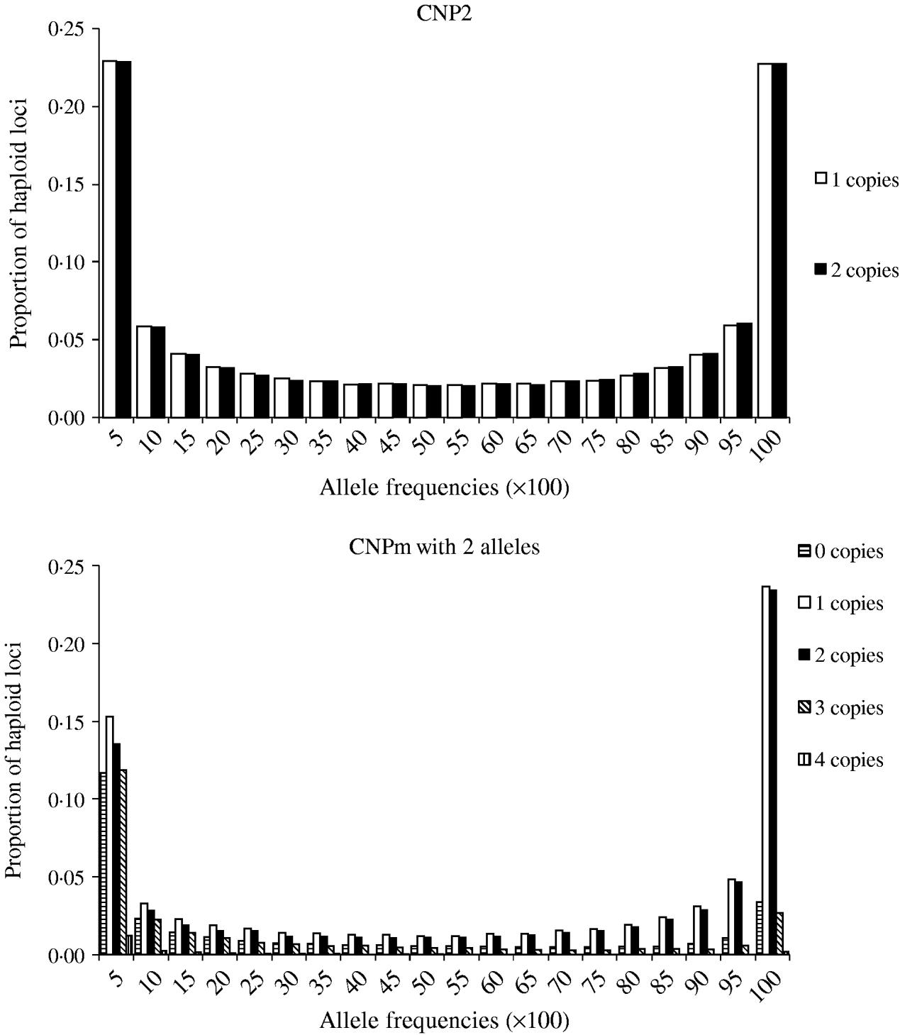
Fig. 2. Average frequencies of alleles across all CNP2 loci and CNPm loci with 2 alleles in generation 4000.
Table 2. Average minor allele frequencies (MAFs) across segregating loci, in ascending order

(ii) Average LD between SNP and CNP loci
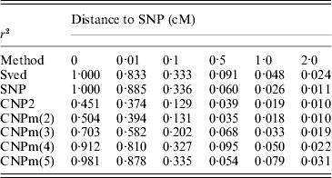
The first set of simulations was also used to calculate LD between different loci at different distances. The average LD between two SNP loci, an SNP and a CNP2 locus and an SNP and a CNPm locus was calculated at all six distances, as well as the expected LD between two SNP loci based on the formula by Sved (Reference Sved1971) (Table 3). The LD between two SNPs was generally close to the expectation. Increased mutation rates, that is CNP2 and CNPm(2) compared to SNP loci, led to lower LD with the nearby SNP and larger deviation of the LD from its expected value. An increase in the number of alleles at the CNPm locus resulted in higher LD with the nearby SNP at all distances.
Table 3. Estimated r2 values between an SNP and an SNP, CNP2 or CNPm loci, and the predicted r2 between two bi-allelic loci according to Sved (Reference Sved1971), located at different distances
(iii) Deterministic R2 values and estimated MSEP of different models
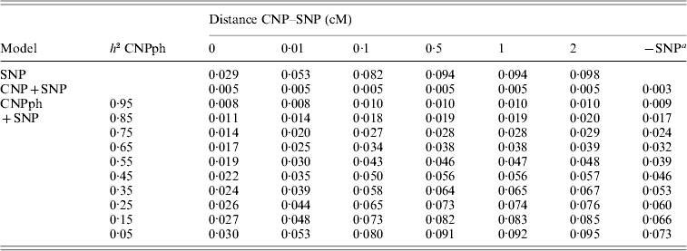
The second set of simulations, based on the haplotype frequencies of the first set, was used to compare deterministically predicted versus obtained model R 2 values. Model R 2 values obtained from analysing the simulated data using models 1, 2, 3, 4 and 5 were similar to those calculated using, respectively, formulae (6), (7), (8), (9) and (10) (Table 4). The small differences are such that generally the R 2 values based on the analysis are smaller than the predicted R 2 values. Only at a distance of 0·0 cM, the model including the SNP and CNP phenotypes always yielded higher R 2 values than the predicted values (Table 4). The R 2 values show that including an SNP in the model, in addition to a CNP phenotype, increases model R 2, when the heritability of the CNP phenotype <0·5, and the distance between the CNP and SNP is short (~<0·5 cM). The predicted R 2 values for models including only CNP phenotypes (using formula (8)) or CNP phenotypes and SNP genotypes (using formula (10)), were plotted as a function of h 2 of the CNP phenotypes for different levels of LD between CNP and SNP loci (Fig. 3). This figure also shows that the gain in R 2 due to including the SNP locus was substantial, depending on the r 2 between the SNP and CNP loci.
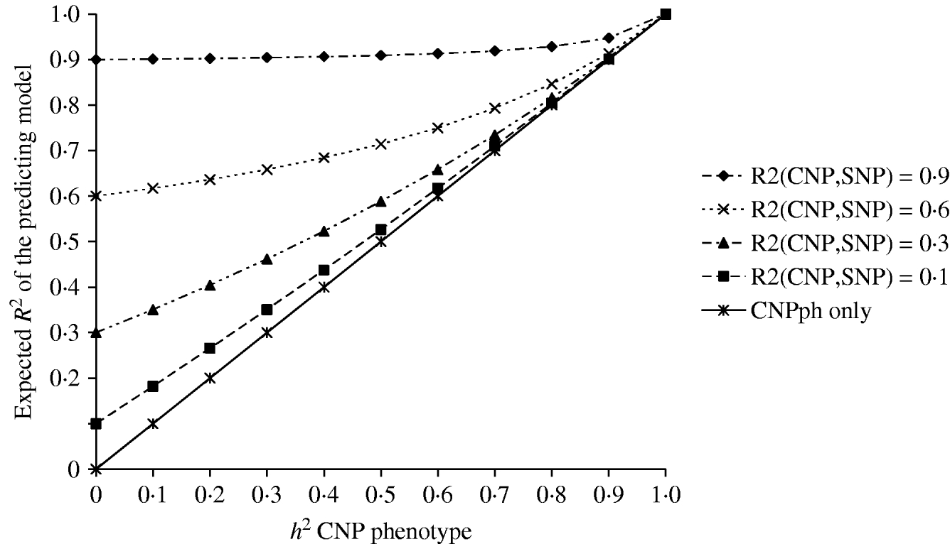
Fig. 3. Deterministic R 2 values obtained for models including CNP phenotypes and SNP genotypes assuming different r 2 values between CNP and SNP loci, as a function of h2 of the CNP phenotypes.
Table 4. Realized and predicted model R2 values for different models averaged across 1000 replicates
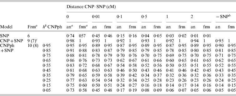
a Predicted using the formulae (frm) or analysis of simulated data (an).
b The same model, but without the SNP. Values are averaged across all 6000 replicates (1000 per distance) for the values based on analysis of simulated data.
c The formula in brackets indicates the formula used for the last column (−SNP).
The MSEP across models 1–5 was clearly largest (i.e. the bias was greatest) when only the SNP genotype or the CNP phenotype with very low h 2 (with or without the SNP genotype) was included in the model (Table 5). Lowest MSEP was found when only the CNP genotype or the CNP phenotype with very high h 2 was included in the model. Including the SNP genotype in addition to the CNP genotype or phenotype in the model hardly changed the MSEP.
Table 5. MSEP for different models, averaged across 1000 replicates
a The result of this model, with the SNP excluded, averaged across all 6000 replicates.
4. Discussion
The objective of this study was to investigate, both empirically and deterministically, the ability to explain genetic variation resulting from a CNP by including the CNP, either by its genotype or by a continuous derivation thereof, alone or together with a nearby SNP in the model. The model R 2 values from analysing the simulated data were very similar to the values predicted with the deterministic formulae. The results indicated that using CNP phenotypes in the model next to a nearby SNP can increase the power of the model substantially, when CNP genotypes cannot easily be derived. It should be noted that the heritability of the CNP phenotype can be interpreted as the reliability of measuring or predicting the CNP genotype. This means that the presented formulae also apply for situations where CNP genotypes are predicted for groups of individuals with a given reliability, conditional on known CNP genotypes in other related individuals.
(i) r2 (LD) between different loci
In this study, we chose to evaluate LD between a CNP and an SNP locus, because SNPs are nowadays widely used as genetic markers in many species. In our analyses, we limited ourselves to including only one SNP in the model, while for instance in cattle nowadays ~50 000 SNPs are used and in humans ~1 000 000 SNPs are used. At a genome of 30 Morgan in length, this implies an average marker spacing of 1 SNP per 0·06 cM. On the cattle 50 k SNP chip, for Holstein the r 2 between adjacent loci is between 0·15 and 0·20, for an average distance of ~0·06 cM (De Roos et al., Reference De Roos, Hayes, Spelman and Goddard2008; Khatkar et al., Reference Khatkar, Nicholas, Collins, Zenger, Al Cavanagh, Barris, Schnabel, Taylor and Raadsma2008). In our simulation, after interpolation, we here find an r 2 value of ~0·44 between two SNP loci, indicating that our achieved LD within the ranges of considered distances is much higher than LD in the 50 k cattle SNP chip. Applications for cattle data may, however, consider multiple SNPs simultaneously. This would lead to explaining higher proportions of variation at the CNP locus then the expected value of 0·20 based on average LD between the adjacent SNPs, since the SNP with the highest LD with the CNP locus (not necessarily the closest SNP) would predict most phenotypic variance and therefore be favoured in an association study. Note that the presented formulae can easily be extended to include multiple SNPs by including more than one SNP in the vector c and matrix K.
In our simulated data an average r 2 of 0·20, that is the average expected value for the 50 k cattle SNP chip, is expected at a distance of 0·23 cM after interpolation. At this distance, after interpolation the r 2 between an SNP and a CNP locus was at least ~0·2. Using formula (10) indicates that by including the CNP phenotype in this scenario, the model R 2 could be increased from 0·2 to over 0·55, when the heritability of the CNP phenotype is at least 0·5.
Based on the 1 000 000 SNPs currently available on commercial human genotyping products, the expected distance to an unobserved CNP is expected to be on average a maximum of 1·5×10−3 Mb, here assumed to be equal to 1·5×10−3 cM. At such a distance, the r 2 between SNPs in the human genome is ~0·25 (P. Navarro, personal communication). In our simulated data, this level of LD between two SNP loci was found at a distance of ~0·17 cM after interpolation. Using formula (10) indicates that by including the CNP phenotype in this scenario, the model R 2 could be increased from 0·17 to over 0·53, when the heritability of the CNP phenotype is at least 0·5.
The differences between the loci considered here are that CNPm and CNP2 loci have a much higher mutation rate than an SNP locus, while a CNPm locus may have more than two alleles segregating. The results showed that the average LD of a CNPm locus with a nearby SNP always increased with increasing number of segregating alleles at the CNPm locus. The results also showed that loci with a higher mutation rate have lower LD with a linked SNP locus. Some studies have reported that microsatellites and short tandem repeats explain more variation at a nearby locus than SNPs do (Ohashi & Tokunaga, Reference Ohashi and Tokunaga2003; Varilo et al., Reference Varilo, Paunio, Parker, Perola, Meyer, Terwilliger and Peltonen2003; Mueller, Reference Mueller2004; Payseur & Cutter, Reference Payseur and Cutter2006). Both microsatellites and short tandem repeats are comparable to CNP, in the sense that their number of segregating alleles may be larger than two, and that their mutation rate is similar to that of CNP loci. Hinds et al. (Reference Hinds, Kloek, Jen, Chen and Frazer2006) reported similar LD between deletion loci and SNPs compared to pairwise SNP LD. Payseur et al. (Reference Payseur, Place and Weber2008) reported that LD between short-tandem-repeat polymorphisms and SNP loci was lower than pairwise SNP LD, in agreement with our results. Summarized, an increased mutation rate leads to lower LD, when the number of segregating alleles is left unchanged. An increased mutation rate can, however, indirectly lead to increased LD, if it increases the number of segregating alleles. A mutation at a segregating locus may lead to breakdown of LD in the short run. When the mutation stays in the population for a longer time, genetic drift will re-establish LD. When the mutation leads to a new allele that was not segregating yet, our results show that the LD with a nearby SNP eventually ends up being on average higher than with fewer alleles segregating at the locus.
(ii) Using CNP phenotypes instead of CNP genotypes
In the simulated datasets, a range of heritabilities of the CNP phenotypes was considered. This applies to CNP loci whose clusters representing the different genotypes are not sufficiently distinct to allow derivation of discrete genotypes. Locke et al. (Reference Locke, Sharp, McCarroll, McGrath, Newman, Cheng, Schwartz, Albertson, Pinkel, Altshuler and Eichler2006) calculated the heritability of CNP loci in two human subpopulations, for 17 loci per subpopulation, and reported an average heritability of 0·86, while the lowest value was only 0·15. This indicates that the whole range of considered heritabilities in our study may actually be present in real data, albeit that most CNP phenotypes are likely to have a heritability relatively close to 1·0.
The maximum average model R 2 value from a model including only an SNP was 0·74. Based on our results, this means that adding CNP phenotypes increases the model R 2 across all distances when the heritability of the CNP phenotypes is >0·05 (Table 4). To illustrate the relation between CNP genotypes and phenotypes when the heritability of CNP phenotypes is low (0·25 in this example), we simulated 500 individuals with one CNP locus with allele frequencies for 0, 1, 2, 3 and 4 copies as in Table 1 for CNPm(3) loci. Visual inspection of the results indicates that in this case a distinction in discrete CNP genotypes is not possible (Fig. 4). Therefore, in such situations including the raw hybridization or predicted CNP genotype in the model provides an opportunity to investigate whether the CNP locus is associated with a trait or disease of interest.
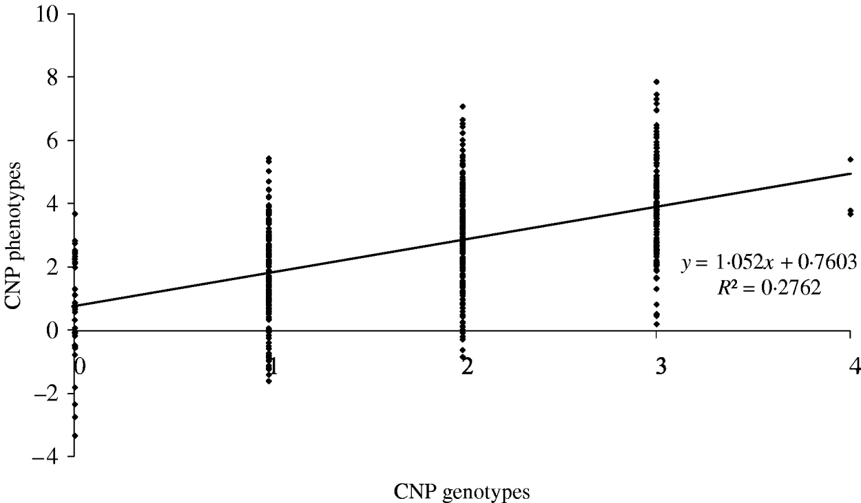
Fig. 4. Simulated CNP phenotypes, assuming a heritability of 0·25, plotted against the CNP genotypes for 500 individuals with a CNP locus with allele frequencies for 0, 1, 2, 3 and 4 copies as in Table 1 for CNPm(3) loci.
(iii) The effect of a CNP locus on the phenotype
In the simulations, it was assumed that the effect of a CNP locus on the phenotype was linearly related with the number of copies at the locus. For practical situations where CNP genotypes cannot be derived, this assumption of linearity allows one to define a general model to test for associations between a CNP locus and a phenotype. Whenever an association is found, the nature of the association can be further investigated by comparing the fit of additional models with non-linear regressions on the CNP phenotype.
Although several studies associate CNP loci with appreciable genetic variation and the expression of genes (e.g. Orozco et al., Reference Orozco, Cokus, Ghazalpour, Ingram-Drake, Wang, van Nas, Che, Araujo, Pellegrini and Lusis2009; Zhang et al., Reference Zhang, Gu, Hurles and Lupski2009), still too little is known to make an estimate of the distribution of effects of CNP loci on the phenotype. The results in Tables 3 and 4 apply to a situation where the CNP genotype explains 10% of the phenotypic variance. Causal effects of most CNP loci are likely to be (much) lower. Consider that the R 2 of predicting an effect of a causal locus, by a linked SNP marker, is equal to the product of the r 2 (LD) between the marker and the causal locus (here: r 2(SNPg,CNPg)) and the squared accuracy of the predicted marker effect (Goddard, Reference Goddard2009). In the derived prediction formulae for the model R 2 values it is assumed that the accuracy of the predicted marker effect is 1·0. For a model including only one locus, the squared accuracy of its estimated effect can be calculated as follows (Daetwyler et al., Reference Daetwyler, Villanueva and Woolliams2008; Goddard, Reference Goddard2009):
where λ=n p/n G, n p is the number of phenotypes (500), n g is the number of effective loci (considering that 1 locus is included in the model) and h2 is the heritability, in this case the variance explained by the CNP locus divided by the phenotypic variance (which reduces to σcnp2). Following this equation, r locus2 is 0·98 for our simulations. Note that the value of 0·98 is somewhat higher still than the obtained model R 2 value for the model including only the CNP genotype (0·95; Table 4). r locus2 would reduce to 0·96 and 0·83, when σcnp2 explains, respectively, 5 or 1% of the total phenotypic variance. This means that when changing σcnp2 to 1% of the phenotypic variance, the obtained model R 2 values for the model only including the CNP or SNP genotype or the CNP phenotype, are expected to be 0·83/0·98=0·85 times the obtained values reported in Table 4. The above formula for r locus2 can also be used to derive the impact of using different numbers of phenotypes in the predictions. Thus, the presented formulae can easily be extended to predict the model R 2 values for different scenarios.
5. Conclusion
The simulations showed that an increased mutation rate leads to lower LD, whereas an increased number of segregating alleles at a locus leads to increased LD.
Under the assumption that x copies at a CNP locus lead to the effect of x times the effect of 1 copy, including the raw hybridizations or predictions of CNP genotypes in the model together with the genotype of a nearby SNP increased power to explain variation at the CNP locus, even when the continuous measure for the CNP explained only 15% of the variation at the CNP locus.
M. P. L. C. thanks John Bastiaansen, Henk Bovenhuis, Mari Smits and Roel Veerkamp for initial discussions on this study, as well as W. G. Hill and two anonymous referees for comments on the performed simulations and earlier versions of the manuscript. The EC-funded Integrated Project SABRE (EC contract number FOOD-CT-2006-01625) is acknowledged for financial support of the stay of M. P. L. C. at the Roslin Institute. D. J. K and C. S. H. acknowledge support from BBSRC through the ISPG grant to the Roslin Institute and the EC-funded Integrated Project SABRE (EC contract number FOOD-CT-2006-01625) D. J. K. additionally acknowledges support from the EC-funded network of excellence EADGENE (EC contract number FOOD-CT-2004-506416) and C. S. H. additionally acknowledges support from the MRC.


