Top-Down NOX Emissions of European Cities Based on the Downwind Plume of Modelled and Space-Borne Tropospheric NO2 Columns

 ,
,  , ,
, ,
Abstract
:1. Background
2. Objectives
3. Datasets
3.1. OMI Tropospheric NO2 Column Retrieval and Processing
3.2. LOTOS-EUROS Datasets
3.3. Surface NO2 Measurements
4. Methods
5. Results and Discussions
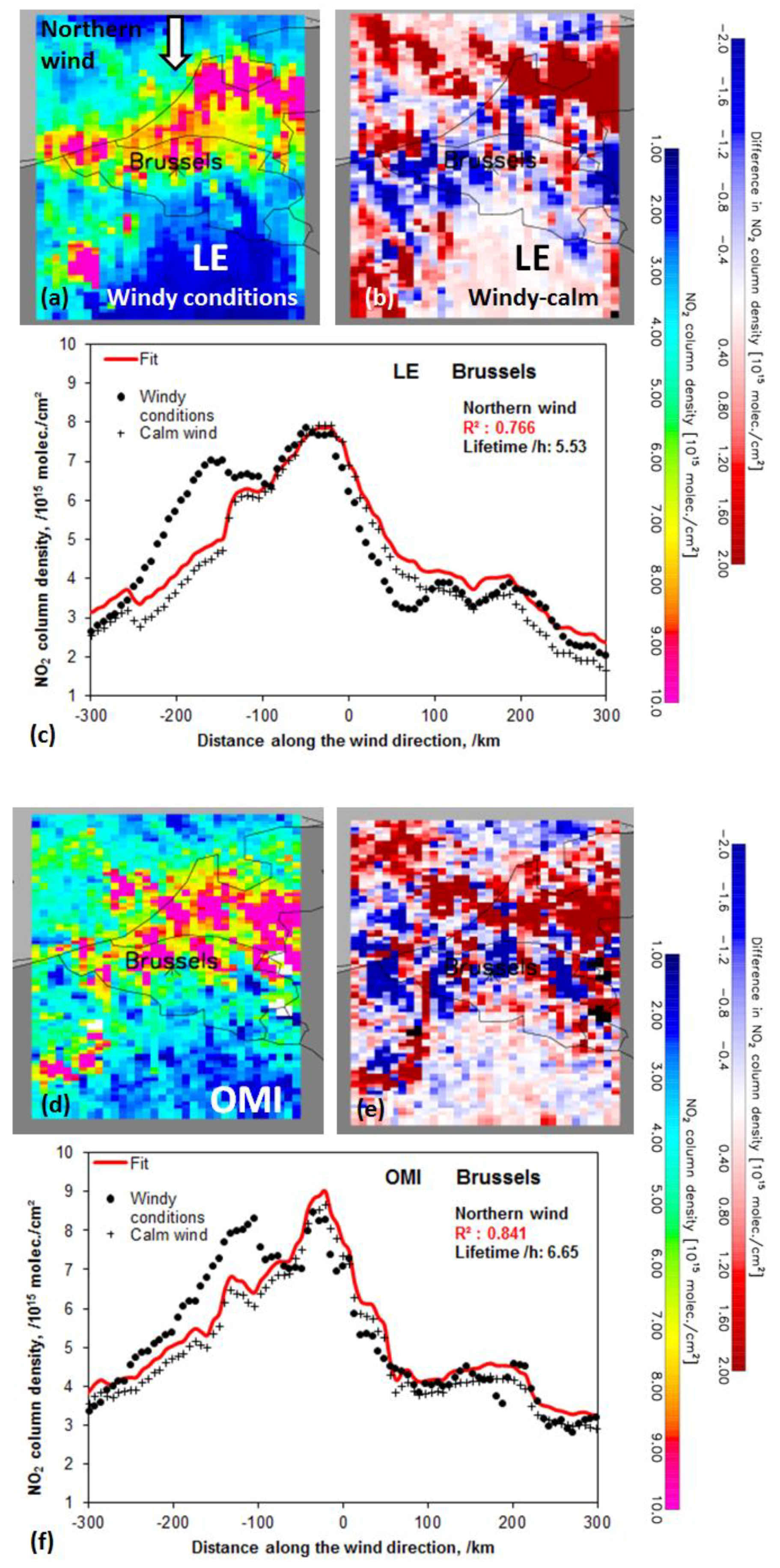
5.1. Lifetimes
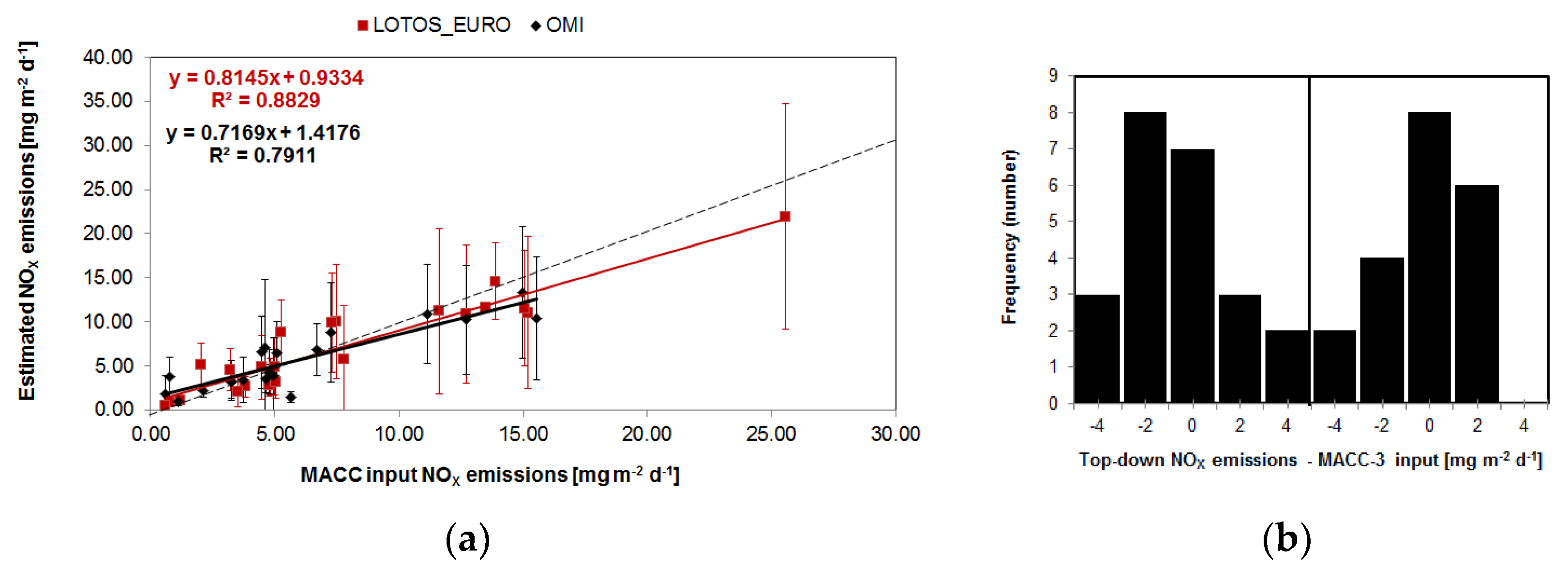
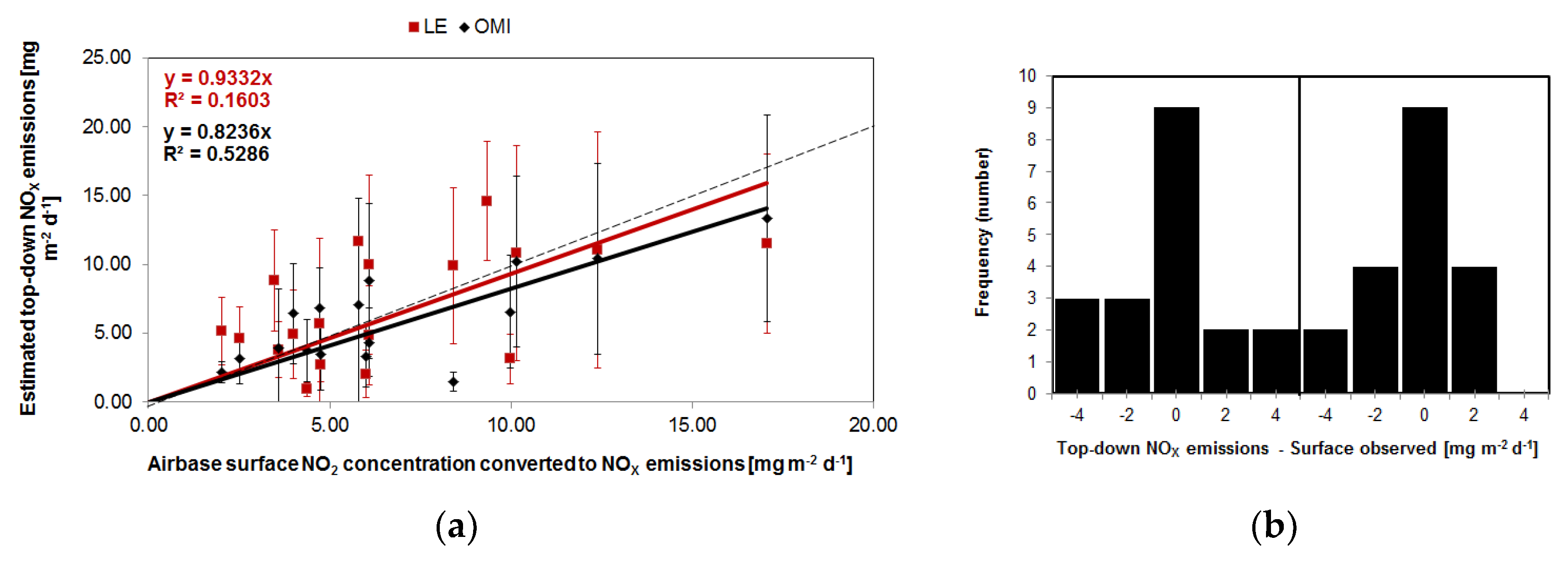
5.2. NOX Emissions
5.3. Uncertainties
6. Summary and Conclusions
Author Contributions
Acknowledgments
Conflicts of Interest
References
- Fischer, P.H.; Marra, M.; Ameling, C.B.; Hoek, G.; Beelen, R.; de Hoogh, K.; Breugelmans, O.; Kruize, H.; Janssen, N.A.; Houthuijs, D. Air Pollution and Mortality in Seven Million Adults: The Dutch Environmental Longitudinal Study (DUELS). Environ. Health Perspect. 2015, 123, 697–704. [Google Scholar] [CrossRef] [PubMed] [Green Version]
- IPCC, 2007: Climate Change 2007: The Physical Science Basis. In Contribution of Working Group I to the Fourth Assessment Report of the Intergovernmental Panel on Climate Change; Solomon, S.; Qin, D.; Manning, M.; Chen, Z.; Marquis, M.; Averyt, K.B.; Tignor, M.; Miller, H.L. (Eds.) Cambridge University Press: Cambridge, UK; New York, NY, USA, 2007. [Google Scholar]
- Arneth, A.; Harrison, S.P.; Zaehle, S.; Tsigaridis, K.; Menon, S.; Bartlein, P.J.; Feichter, J.; Korhola, A.; Kulmala, M.; O’Donnell, D.; et al. Terrestrial biogeochemical feedbacks in the climate system. Nat. Geosci. 2010, 3, 525–532. [Google Scholar] [CrossRef] [Green Version]
- EEA. Air Quality in Europe—2015 Report; EEA Report; European Environment Agency: Copenhagen, Denmark, 2015. [Google Scholar]
- Guerreiro, C.B.B.; Foltescu, V.; de Leeuw, F. Air quality status and trends in Europe. Atmos. Environ. 2014, 98, 376–384. [Google Scholar] [CrossRef] [Green Version]
- Warneck, P. Chemistry of the Natural Atmosphere; Academic Press: San Diego, CA, USA, 1999; p. 757. [Google Scholar]
- Mollner, A.K.; Valluvadasan, S.; Feng, L.; Sprague, M.K.; Okumura, M.; Milligan, D.B.; Bloss, W.J.; Sander, S.P.; Martien, P.T.; Harley, R.A.; et al. Rate of gas phase association of hydroxyl radical and nitrogen dioxide. Science 2010, 330, 646–649. [Google Scholar] [CrossRef] [PubMed]
- Butler, T.M.; Lawrence, M.G.; Gurjar, B.R.; Van Aardenne, J.; Schultz, M.; Lelieveld, J. The representation of emissions from megacities in global emission inventories. Atmos. Environ. 2008, 42, 703–719. [Google Scholar] [CrossRef]
- EDGAR. Available online: http://themasites.pbl.nl/en/themasites/edgar/documentation/uncertainties/index.html (accessed on 29 July 2018).
- Beirle, S.; Boersma, K.F.; Platt, U.; Lawrence, M.G.; Wagner, T. Megacity emissions and lifetimes of nitrogen oxides probed from space. Science 2011, 333, 1737–1739. [Google Scholar] [CrossRef] [PubMed]
- Cames, M.; Helmers, E. Critical evaluation of the European diesel car boom-global comparison, environmental effects and various national strategies. Environ. Sci. Eur. 2013. [Google Scholar] [CrossRef]
- Smith, S.J.; Zhou, Y.; Kyle, P.; Wang, H.; Yu, H. A Community Emissions Data System (CEDS): Emissions for CMIP6 and Beyond. In Proceedings of the 2015 International Emission Inventory Conference, San Diego, CA, USA, 12–16 April 2015. [Google Scholar]
- Castellanos, P.; Boersma, K.F. Reductions in nitrogen oxides over Europe driven by environmental policy and economic recession. Sci. Rep. 2012, 2. [Google Scholar] [CrossRef] [PubMed]
- Ialongo, I.; Hakkarainen, J.; Hyttinen, N.; Jalkanen, J.-P.; Johansson, L.; Boersma, K.F.; Krotkov, N.; Tamminen, J. Characterization of OMI tropospheric NO2 over the Baltic Sea region. Atmos. Chem. Phys. 2014, 14, 7795–7805. [Google Scholar] [CrossRef]
- Lu, Z.; Streets, D.G.; de Foy, B.; Lamsal, L.N.; Duncan, B.N.; Xing, J. Emissions of nitrogen oxides from US urban areas: estimation from Ozone Monitoring Instrument retrievals for 2005–2014. Atmos. Chem. Phys. 2015, 15, 10367–10383. [Google Scholar] [CrossRef]
- Liu, F.; Beirle, S.; Zhang, Q.; Dörner, S.; He, K.; Wagner, T. NOx lifetimes and emissions of cities and power plants in polluted background estimated by satellite observations. Atmos. Chem. Phys. 2016, 16, 5283–5298. [Google Scholar] [CrossRef]
- Lamsal, L.N.; Martin, R.V.; Padmanabhan, A.; van Donkelaar, A.; Zhang, Q.; Sioris, C.E.; Chance, K.; Kurosu, P.; Newchurch, M.J. Application of satellite observations for timely updates to global anthropogenic NOx emission inventories. Geophys. Res. Lett. 2011, 38. [Google Scholar] [CrossRef]
- Lin, J.-T.; McElroy, M.B. Detection from space of a reduction in anthropogenic emissions of nitrogen oxides during the Chinese economic downturn. Atmos. Chem. Phys. 2011, 11, 8171–8188. [Google Scholar] [CrossRef] [Green Version]
- Valin, L.C.; Russell, A.R.; Cohen, R.C. Variations of OH radical in an urban plume inferred from NO2 column measurements. Geophys. Res. Lett. 2013, 40, 1856–1860. [Google Scholar] [CrossRef]
- Vinken, G.C.M.; Boersma, K.F.; van Donkelaar, A.; Zhang, L. Constraints on ship NOx emissions in Europe using GEOS-Chem and OMI satellite NO2 observations. Atmos. Chem. Phys. 2014, 14, 1353–1369. [Google Scholar] [CrossRef]
- Boersma, K.F.; Vinken, G.C.M.; Tournadre, J. Ships going slow in reducing their NOx emissions: Changes in 2005–2012 ship exhaust inferred from satellite measurements over Europe. Environ. Res. Lett. 2015, 10, 074007. [Google Scholar] [CrossRef]
- Verstraeten, W.W.; Neu, J.L.; Williams, J.E.; Bowman, K.W.; Worden, J.R.; Boersma, K.F. Rapid increases in tropospheric ozone production and export from China. Nat. Geosci. 2015, 8. [Google Scholar] [CrossRef]
- Miyazaki, K.; Eskes, H.; Sudo, K.; Boersma, K.F.; Bowman, K.; Kanaya, Y. Decadal changes in global surface NOx emissions from multi-constituent satellite data assimilation. Atmos. Chem. Phys. 2017, 2, 807–837. [Google Scholar] [CrossRef]
- Lin, J.-T.; Liu, Z.; Zhang, Q.; Liu, H.; Mao, J.; Zhuang, G. Modeling uncertainties for tropospheric nitrogen dioxide columns affecting satellite-based inverse modeling of nitrogen oxides emissions. Atmos. Chem. Phys. 2012, 12, 12255–12275. [Google Scholar] [CrossRef] [Green Version]
- Stavrakou, T.; Müller, J.-F.; Boersma, K.F.; Van der A, R.J.; Kurokawa, J.; Ohara, T.; Zhang, Q. Key chemical NOx sink uncertainties and how they influence top-down emissions of nitrogen oxides. Atmos. Chem. Phys. 2013, 13, 9057–9082. [Google Scholar] [CrossRef]
- Ye, C.; Zhou, X.; Pu, D.; Stutz, J.; Festa, J.; Spolaor, M.; Tsai, C.; Cantrell, C.; Mauldin, R.L.; Campos, T.; et al. Rapid cycling of reactive nitrogen in the marine boundary layer. Nature 2016, 532, 489–491. [Google Scholar] [CrossRef] [PubMed]
- Schaap, M.; Timmermans, R.M.A.; Roemer, M.; Boersen, G.A.C.; Builtjes, P.J.H.; Sauter, F.J.; Velders, G.J.M.; Beck, J.P. The LOTOS-EUROS Model: Description, validation and latest developments. Int. J. Environ. Pollut. 2008, 32, 270–290. [Google Scholar] [CrossRef]
- Kuenen, J.J.P.; Visschedijk, A.J.H.; Jozwicka, M.; Denier van der Gon, H.A.C. TNO-MACC_II emission inventory; a multi-year (2003–2009) consistent high-resolution European emission inventory for air quality modelling. Atmos. Chem. Phys. 2014, 14, 10963–10976. [Google Scholar] [CrossRef]
- Boersma, K.F.; Eskes, H.J.; Dirksen, R.J.; van der A, R.J.; Veefkind, J.P.; Stammes, P.; Huijnen, V.; Kleipool, Q.L.; Sneep, M.; Claas, J.; et al. An improved tropospheric NO2 column retrieval algorithm for the Ozone Monitoring Instrument. Atmos. Meas. Tech. 2011, 4, 1905–1928. [Google Scholar] [CrossRef]
- Dirksen, R.J.; Boersma, K.F.; Eskes, H.J.; Ionov, D.V.; Bucsela, E.J.; Levelt, P.F.; Kelder, H.M. Evaluation of stratospheric NO2 retrieved from the Ozone Monitoring Instrument: intercomparison, diurnal cycle and trending. J. Geophys. Res. 2011, 116, D08305. [Google Scholar] [CrossRef]
- Boersma, K.F.; Jacob, D.J.; Trainic, M.; Rudich, Y.; De Smedt, I.; Dirksen, R.; Eskes, H.J. Validation of urban NO2 concentrations and their diurnal and seasonal variations observed from the SCIAMACHY and OMI sensors using in situ surface measurements in Israeli cities. Atmos. Chem. Phys. 2009, 9, 3867–3879. [Google Scholar] [CrossRef] [Green Version]
- Lin, J.-T.; Martin, R.V.; Boersma, K.F.; Sneep, M.; Stammes, P.; Spurr, R.; Wang, P.; Van Roozendael, M.; Clémer, K.; Irie, H. Retrieving tropospheric nitrogen dioxide from the Ozone Monitoring Instrument: Effects of aerosols, surface reflectance anisotropy and vertical profile of nitrogen dioxide. Atmos. Chem. Phys. 2014, 14, 1441–1461. [Google Scholar] [CrossRef] [Green Version]
- Irie, H.; Boersma, K.F.; Kanaya, Y.; Takashima, H.; Pan, X.; Wang, Z.F. Quantitative bias estimates for tropospheric NO2 columns retrieved from SCIAMACHY, OMI and GOME-2 using a common standard for East Asia. Atmos. Meas. Tech. 2012, 5, 2403–2411. [Google Scholar] [CrossRef]
- Flemming, J.; Inness, A.; Flentje, H.; Huijnen, V.; Moinat, P.; Schultz, M.G.; Stein, O. Coupling global chemistry transport models to ECMWF’s integrated forecast system. Geosci. Model Dev. Discuss. 2009, 2, 763–795. [Google Scholar] [CrossRef]
- Lin, J.-T. Satellite constraint for emissions of nitrogen oxides from anthropogenic, lightning and soil sources over East China on a high-resolution grid. Atmos. Chem. Phys. 2012, 12, 2881–2898. [Google Scholar] [CrossRef] [Green Version]
- Acarreta, J.R.; de Haan, J.F.; Stammes, P. Cloud pressure retrieval using the O2-O2 absorption band at 477 nm. J. Geophys. Res. 2004, 109, D05204. [Google Scholar] [CrossRef]
- Dee, D.P.; Uppala, S.M.; Simmons, A.J.; Berrisford, P.; Poli, P.; Kobayashi, S.; Andrae, U.; Balmaseda, M.A.; Balsamo, G.; Bauer, P.; et al. The ERA-Interim reanalysis: configuration and performance of the data assimilation system. Q. J. R. Meteorol. Soc. 2011, 137, 553–597. [Google Scholar] [CrossRef] [Green Version]
- Duncan, B.N.; Lamsal, L.N.; Thompson, A.M.; Yoshida, Y.; Lu, Z.; Streets, D.G.; Hurwitz, M.M.; Pickering, K.E. A space-based, high-resolution view of notable changes in urban NOx pollution around the world (2005–2014). J. Geophys. Res. Atmos. 2016, 121, 976–996. [Google Scholar] [CrossRef]
- Elansky, N.F.; Lavrova, O.V.; Skorokhod, A.I.; Belikov, I.B. Trace gases in the atmosphere over Russian cities. Atmos. Environ. 2016, 143, 108–119. [Google Scholar] [CrossRef]
- Olivier, J.G.J.; Janssens-Maenhout, G.; Muntean, M.; Peters, J.A.H.W. Trends in Global CO2 Emissions: 2014 Report; ©PBL Netherlands Environmental Assessment Agency: The Hague, The Netherlands, 2014. [Google Scholar]
- De Foy, B.; Lu, Z.; Streets, D.G.; Lamsal, L.N.; Duncan, B.N. Estimates of power plant NOx emissions and lifetimes from OMI NO2 satellite retrievals. Atmos. Environ. 2015, 116, 1–11. [Google Scholar] [CrossRef]


| OMI | LE | |||||||
|---|---|---|---|---|---|---|---|---|
| Lat | Lon | Lifetime | Top-down E | MACC E | Lifetime | Top-down E | MACC E | |
| (N) | (E) | (h) | (mg m−2 d−1) | (mg m−2 d−1) | (h) | (mg m−2 d−1) | (mg m−2 d−1) | |
| Mean | 4.1 ± 2.2 | 5.55 ± 3.49 | 7.17 ± 3.80 | 3.7 ± 2.2 | 7.11 ± 4.03 | 7.59 ± 3.97 | ||
| Stdev | 1.3 ± 0.7 | 3.48 ± 2.29 | 6.29 ± 5.50 | 1.0 ± 0.9 | 5.28 ± 3.36 | 6.09 ± 5.37 | ||
| Helsinki | 60.16 | 24.93 | 4.7 ± 2.1 | 3.88 ± 4.35 | 4.97 ± 1.62 | 3.1 ± 1.6 | 3.78 ± 2.03 | 4.81 ± 1.70 |
| St-Petersburg | 59.93 | 30.31 | 3.9 ± 1.5 | 4.28 ± 1.65 | 27.02 ± 26.25 | 3.8 ± 2.2 | 21.95 ± 12.79 | 25.57 ± 25.26 |
| Edinburgh | 55.94 | −3.19 | 4.2 ± 1.8 | 6.81 ± 2.92 | 6.67 ± 2.30 | 4.8 ± 5.1 | 5.71 ± 6.16 | 7.78 ± 2.59 |
| Moscow | 55.75 | 37.61 | 5.4 ± 2.8 | 10.91 ± 5.62 | 11.12 ± 2.67 | 4.1 ± 3.4 | 11.21 ± 9.34 | 11.64 ± 2.21 |
| Amsterdam | 52.37 | 4.89 | 2.8 ± 1.7 | 10.41 ± 6.94 | 15.56 ± 3.88 | 3.0 ± 2.3 | 11.04 ± 8.59 | 15.19 ± 4.25 |
| Warsaw | 52.22 | 22.01 | 2.9 ± 1.8 | 3.74 ± 2.28 | 0.75 ± 0.03 | 3.7 ± 2.0 | 0.90 ± 0.48 | 0.76 ± 0.02 |
| London | 51.50 | −0.13 | 4.6 ± 2.5 | 13.33 ± 7.50 | 14.97 ± 10.81 | 3.0 ± 1.7 | 11.52 ± 6.54 | 15.08 ± 10.93 |
| Antwerp | 51.25 | 4.38 | 4.4 ± 2.6 | 10.22 ± 6.20 | 12.73 ± 3.19 | 2.9 ± 2.0 | 10.85 ± 7.82 | 12.73 ± 3.19 |
| Brussels | 50.83 | 4.33 | 4.8 ± 2.3 | 6.42 ± 3.66 | 5.09 ± 2.15 | 3.8 ± 2.5 | 4.90 ± 3.23 | 4.98 ± 1.95 |
| Kiev | 50.45 | 30.52 | 5.4 ± 2.1 | 3.56 ± 1.63 | 4.64 ± 0.73 | 3.9 ± 1.6 | 2.74 ± 1.13 | 4.76 ± 0.60 |
| Prague | 50.07 | 14.43 | 3.3 ± 2.5 | 3.44 ± 2.60 | 3.73 ± 1.72 | 3.7 ± 1.6 | 2.66 ± 1.17 | 3.82 ± 1.69 |
| Krakow | 50.06 | 19.94 | 2.9 ± 1.8 | 6.56 ± 4.09 | 4.49 ± 3.15 | 2.9 ± 1.6 | 3.12 ± 1.80 | 5.02 ± 3.49 |
| Paris | 48.85 | 2.35 | 2.7 ± 1.7 | 8.80 ± 5.66 | 7.25 ± 5.98 | 3.7 ± 2.4 | 9.98 ± 6.50 | 7.46 ± 5.06 |
| Vienna | 48.20 | 16.37 | 7.7 ± 3.3 | 1.45 ± 0.66 | 5.66 ± 4.16 | 5.8 ± 2.5 | 9.91 ± 5.67 | 7.32 ± 4.97 |
| Budapest | 47.57 | 19.11 | 2.9 ± 1.8 | 3.31 ± 2.25 | 3.24 ± 0.65 | 2.6 ± 2.2 | 2.03 ± 1.72 | 3.50 ± 0.29 |
| Milan | 45.46 | 9.19 | 3.8 ± 1.1 | / | 5.24 ± 0.76 | 3.9 ± 1.2 | 8.85 ± 3.67 | 5.24 ± 0.56 |
| Bucharest | 44.43 | 26.10 | 3.6 ± 4.0 | 1.83 ± 2.01 | 0.59 ± 0.10 | 2.3 ± 1.9 | 0.51 ± 0.43 | 0.59 ± 0.10 |
| Marseille | 43.29 | 5.37 | 3.4 ± 1.7 | / | 15.40 ± 6.70 | 4.1 ± 1.2 | 14.60 ± 4.31 | 13.88 ± 6.92 |
| Rome | 41.89 | 12.51 | 1.8 ± 2.0 | 7.06 ± 7.73 | 4.61 ± 1.55 | 3.5 ± 2.2 | 11.67 ± 0.35 | 13.49 ± 7.17 |
| Naples | 40.85 | 14.26 | 3.1 ± 1.8 | 3.16 ± 1.85 | 3.25 ± 2.59 | 3.4 ± 1.7 | 4.57 ± 2.34 | 3.23 ± 2.62 |
| Thessaloniki | 40.63 | 22.94 | 4.5 ± 1.4 | 2.19 ± 0.77 | 2.10 ± 1.02 | 2.1 ± 1.0 | 5.15 ± 2.44 | 2.02 ± 0.93 |
| Madrid | 40.41 | −3.70 | 5.7 ± 3.3 | 4.32 ± 2.48 | 4.75 ± 5.03 | 4.6 ± 3.4 | 4.85 ± 3.62 | 4.45 ± 4.47 |
| Istanbul | 40.00 | 28.97 | 4.5 ± 2.2 | 0.94 ± 0.48 | 1.12 ± 0.38 | 6.4 ± 2.3 | 1.13 ± 0.48 | 1.18 ± 0.38 |
© 2018 by the authors. Licensee MDPI, Basel, Switzerland. This article is an open access article distributed under the terms and conditions of the Creative Commons Attribution (CC BY) license (http://creativecommons.org/licenses/by/4.0/).
Share and Cite
Verstraeten, W.W.; Boersma, K.F.; Douros, J.; Williams, J.E.; Eskes, H.; Liu, F.; Beirle, S.; Delcloo, A. Top-Down NOX Emissions of European Cities Based on the Downwind Plume of Modelled and Space-Borne Tropospheric NO2 Columns. Sensors 2018, 18, 2893. https://doi.org/10.3390/s18092893
Verstraeten WW, Boersma KF, Douros J, Williams JE, Eskes H, Liu F, Beirle S, Delcloo A. Top-Down NOX Emissions of European Cities Based on the Downwind Plume of Modelled and Space-Borne Tropospheric NO2 Columns. Sensors. 2018; 18(9):2893. https://doi.org/10.3390/s18092893
Chicago/Turabian StyleVerstraeten, Willem W., Klaas Folkert Boersma, John Douros, Jason E. Williams, Henk Eskes, Fei Liu, Steffen Beirle, and Andy Delcloo. 2018. "Top-Down NOX Emissions of European Cities Based on the Downwind Plume of Modelled and Space-Borne Tropospheric NO2 Columns" Sensors 18, no. 9: 2893. https://doi.org/10.3390/s18092893