
Using Space-Time Features to Improve Detection of Forest Disturbances from Landsat Time Series


Laboratory of Geo-Information Science and Remote Sensing, Wageningen University & Research, Droevendaalsesteg 3, 6708 PB Wageningen, The Netherlands
*
Author to whom correspondence should be addressed.
Remote Sens. 2017, 9(6), 515; https://doi.org/10.3390/rs9060515
Submission received: 2 March 2017
/
Revised: 18 May 2017
/
Accepted: 21 May 2017
/
Published: 23 May 2017
Abstract
:Current research on forest change monitoring using medium spatial resolution Landsat satellite data aims for accurate and timely detection of forest disturbances. However, producing forest disturbance maps that have both high spatial and temporal accuracy is still challenging because of the trade-off between spatial and temporal accuracy. Timely detection of forest disturbance is often accompanied by many false detections, and existing approaches for reducing false detections either compromise the temporal accuracy or amplify the omission error for forest disturbances. Here, we propose to use a set of space-time features to reduce false detections. We first detect potential forest disturbances in the Landsat time series based on two consecutive negative anomalies, and subsequently use space-time features to confirm forest disturbances. A probability threshold is used to discriminate false detections from forest disturbances. We demonstrated this approach in the UNESCO Kafa Biosphere Reserve located in the southwest of Ethiopia by detecting forest disturbances between 2014 and 2016. Our results show that false detections are reduced significantly without compromising temporal accuracy. The user’s accuracy was at least 26% higher than the user’s accuracies obtained when using only temporal information (e.g., two consecutive negative anomalies) to confirm forest disturbances. We found the space-time features related to change in spatio-temporal variability, and spatio-temporal association with non-forest areas, to be the main predictors for forest disturbance. The magnitude of change and two consecutive negative anomalies, which are widely used to distinguish real changes from false detections, were not the main predictors for forest disturbance. Overall, our findings indicate that using a set of space-time features to confirm forest disturbances increases the capacity to reject many false detections, without compromising the temporal accuracy.
1. Introduction
Current research on forest change monitoring aims for accurate and timely detection of forest disturbances. Many change detection approaches have therefore been proposed in recent years to improve the detection of forest disturbances from medium spatial resolution satellite data (e.g., Landsat) [1,2,3,4,5,6,7,8]. The proposed approaches have addressed many key challenges, including seasonality in dry forests [9,10,11]. However, it is still challenging to produce forest disturbance maps which have both high spatial and temporal accuracy; there is always a trade-off [1,6,7,10]. A shorter temporal detection delay is typically associated with high producer’s accuracy and low user‘s accuracy [10]. Low user’s accuracy implies that timely detection of forest disturbances is accompanied by many false detections. False detections in satellite time series may occur because of insufficient deseasonalisation or because of the presence of sensors’ artefacts and remnant atmospheric contaminations [1,12]. Yet, existing approaches lack the capacity to reject false detections without compromising the temporal accuracy. In cases where high user’s accuracy has been reported, the omission error for small-scale forest disturbances was high [8]. In short, amplified false detections and high omission error for small-scale forest disturbances are two major challenges that currently hinder accurate and timely detection of forest disturbances.
Recent studies attempted to remedy the problem of false detections by using a threshold on the magnitude of change to discriminate real disturbances from false detections [9,13]. The use of a threshold on the magnitude of change is based on the assumption that, when compared to real changes, false detections have a smaller magnitude of change. This assumption is problematic, however, because forest disturbances that involve partial removal of forest cover may also have a small magnitude of change [14]. Small-scale and gradual forest disturbances, which are common especially in Africa and caused mainly by small-holder agriculture expansion, domestic firewood and charcoal extractions [15], also tend to have a small magnitude of change [13]. Recent studies show that false detections are particularly common in areas where small-scale forest disturbances, caused by small-holder agriculture and human settlements expansion, are prevalent [16]. Separating forest disturbances from false detections using a threshold on the magnitude of change in such areas may therefore lead to high omission error for small-scale forest disturbances. The difficulty in separating false detections and forest disturbances may explain why small-scale forest disturbances are still a major constraint to accurate mapping and quantification of forest loss [17]. It is therefore important that new change detection approaches improve the detection of small-scale forest disturbances in order to achieve accurate mapping and quantification of forest loss.
Alternative to magnitude of change, some change detection approaches use consecutive anomalies to confirm forest disturbance. Essentially, forest disturbance is only confirmed if there are at least two or more consecutive negative anomalies in the time series [3,6,7,8]. An observation is considered a negative anomaly if it is below a specified threshold [18]. The approach of consecutive anomalies is based on the assumption that the presence of multiple consecutive negative anomalies in the time series may be a strong indicator of forest disturbance because the impact of forest disturbances are typically persistent through time [1]. Consecutive negative anomalies are also considered more robust against noise in the time series than a threshold on the magnitude of change [1,3,7]. When detecting forest disturbances in a timely manner using a consecutive negative anomaly approach, however, a threshold for defining an observation as an anomaly has to be less strict [6,10]. Unfortunately, a less strict threshold amplifies false detections [6]. In addition to consecutive anomalies, other approaches use temporal metrics derived from pixel-time series of Landsat spectral bands and indices to calculate the likelihood of forest loss [8]. Forest loss is confirmed when there are two consecutive observations at the pixel showing a higher likelihood of forest loss [8]. This approach is particularly novel because the likelihood of forest loss is calculated based on a set of spectral and temporal metrics. Overall, this forest change detection approach produced a forest disturbance map with high user’s accuracy in Peru, but the omission error for small-scale forest disturbances was high [8].
Solving the problems of false detections and omission of small-scale forest disturbances remains challenging mainly because existing forest change detection approaches only rely on temporal and spectral information; they ignore spatial information. Yet, forest disturbances, by default, are spatio-temporal processes [19]. Oftentimes, new disturbances, especially those induced by humans, have both a spatial and temporal association to old disturbances [19]. This spatio-temporal association arises because new loggings, for example, are more likely to occur within the neighbourhood of previously logged areas or logging routes than in areas which are far from previous disturbances. Essentially, a set of “space-time features” can be extracted from satellite data cubes and they can subsequently be used as indicators for forest disturbance in order to discriminate false detections from real disturbances. To the best of our knowledge, this idea of using space-time features to discriminate false detections from real disturbances has not yet been investigated.
The objective of this paper was to investigate whether the detection of forest disturbances from Landsat time series can be improved by using space-time features. We propose a new approach that first detects potential forest disturbances in the pixel-time series based on two-consecutive negative anomalies, and we subsequently use space-time features to confirm forest disturbances. The forest disturbance maps generated using the space-time features approach were compared to maps generated using two-consecutive negative anomaly only to detect forest disturbances, and using two-consecutive negative anomalies and the magnitude of change to confirm forest disturbances. We hypothesised that the space-time features approach would produce forest disturbance maps which are spatially more accurate. Throughout this paper, forest disturbance is defined as forest loss which constitutes either full or partial removal of forest cover, which is visible from Landsat multi-spectral data.
2. Study Area
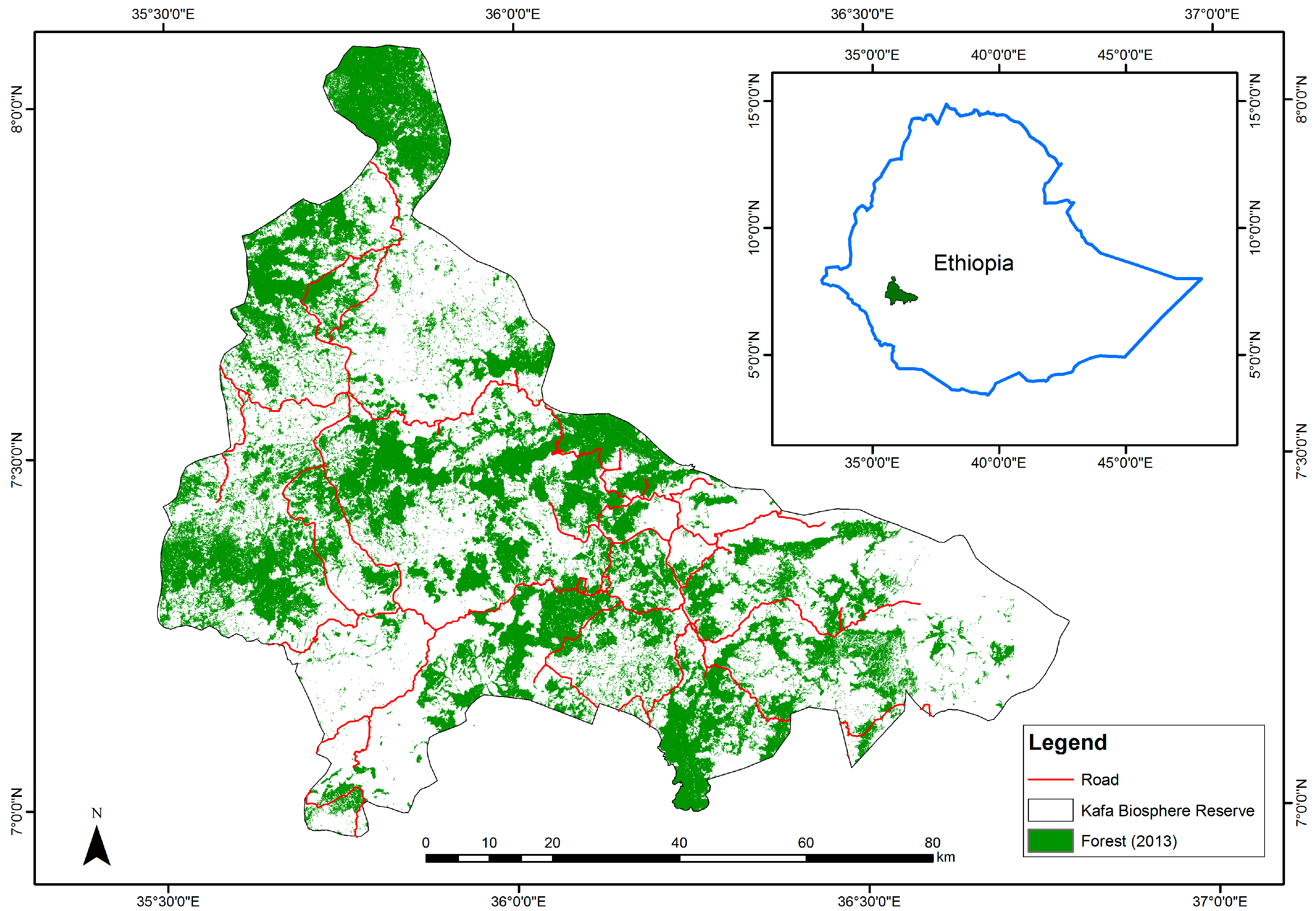
Our study focused on detecting forest disturbances in the UNESCO Kafa Biosphere Reserve, situated in the southwest of Ethiopia (Figure 1), where a moist Afromontane broadleaf evergreen forest with moderate seasonality exists [13]. The forest in this area is subject to small-scale and gradual disturbance processes, caused mainly by small-holder agriculture, human settlements expansion, industrial coffee plantations, and domestic firewood and charcoal extractions [20,21]. Previous studies in the UNESCO Kafa Biosphere Reserve show that separating forest disturbances from false detections is difficult, especially those that involve partial removal of the forest cover [13,16,22]. This study area is therefore ideal for evaluating the importance of using space-time features to achieve accurate and timely detection of forest disturbances. We defined forest disturbance as full or partial removal of forest cover, which is visible from Landsat multi-spectral images.
3. Data and Methods
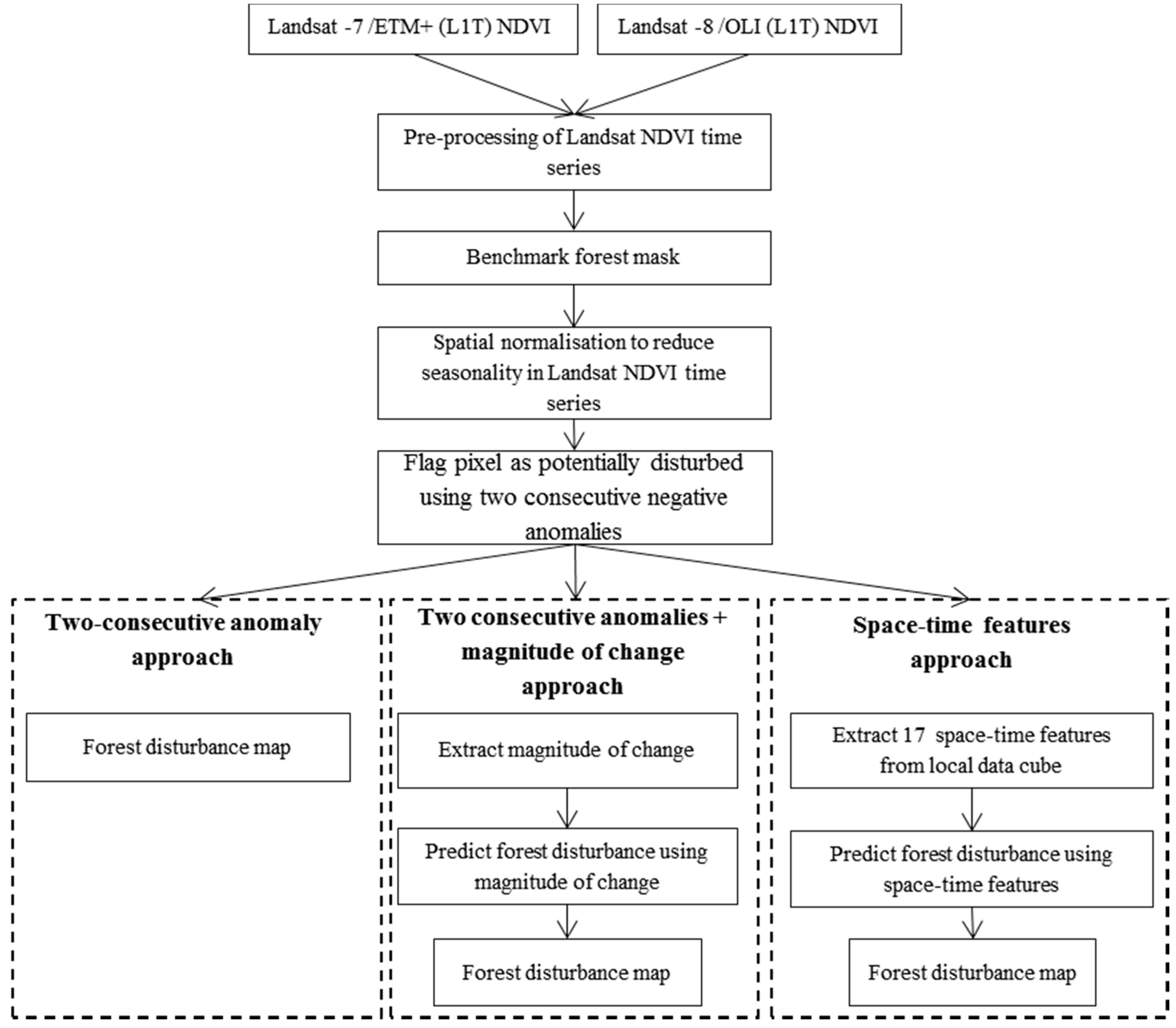
Figure 2 provides the overview of the data used, and the methods followed. To detect forest disturbances, we first pre-processed a total of 172 terrain corrected (L1T) multi-spectral images from Landsat-7 Enhanced Thematic Mapper (ETM+, 116 images) and Landsat-8 Operational Land Imager (OLI, 56 images) acquired between January 2010 and June 2016. From these images, we derived a normalised difference vegetation index (NDVI; [23,24], Section 3.1.1). Second, we produced a benchmark forest mask (Section 3.1.2), and used it to mask non-forest areas in the NDVI time series. Third, we normalised NDVI time series spatially to reduce seasonality (Section 3.1.3). Fourth, we flagged pixels with two consecutive negative anomalies in Landsat NDVI time series as potentially disturbed (Section 3.2). Fifth, we used three different approaches to confirm forest disturbance (Section 3.3). In the first approach (Section 3.3.1), forest disturbances were immediately confirmed once there were two consecutive negative anomalies in the pixel-time series (Two-consecutive anomaly approach). In the second approach (Section 3.3.2), we used two consecutive negative anomalies and the magnitude of change to calculate the probability of forest disturbance (Two consecutive anomalies + magnitude of change approach). In the third approach (Section 3.3.3), we used several space-time features from the local data cube of a flagged pixel to calculate the probability of forest disturbance (Space-time feature approach). Finally, for each approach, we estimated the spatial and temporal accuracy for forest disturbance maps (Section 3.4).
3.1. Pre-Processing Steps
3.1.1. Landsat NDVI
Landsat NDVI time series was derived from terrain corrected (L1T) Landsat-7/ETM+ and Landsat-8/OLI images, spanning from January 2010 to June 2016. Landsat-7/ETM+ and Landsat-8/OLI images, geometrically and atmospherically corrected, were obtained from The United State of America’s Geological Survey (USGS) Landsat surface Reflectance (SR) Climate Data Records (CDR; http://landsat.usgs.gov/CDR_LSR.php). USGS use Landsat Ecosystem Disturbance Adaptive Processing System (LEDAPS) algorithm [25] to generate Landsat-7/ETM+ surface reflectance products. Landsat 8 OLI surface reflectance products are generated using Landsat 8 OLI surface reflectance algorithm [26]. Clouds and cloud shadows in Landsat-7/ETM+ and Landsat-8/OLI images were masked using the CFmask cloud-shadow mask product [27]. CFmask products are distributed together with the Landsat SR CDR Products. Our reference period was 2010–2013, whereas the monitoring period was 2014–2016.
3.1.2. Benchmark Forest Mask
A benchmark forest mask is essential when monitoring forest cover disturbances from satellite time series in order to avoid confusing forest cover loss with other land cover dynamics (e.g., cropping cycles; [9,13]). Similar to [13], we used a supervised maximum likelihood classifier to generate a forest mask from Landsat-8 OLI multi-spectral image time series for 2013. In UNESCO Kafa Biosphere Reserve, there are complex patchy mosaic transitional areas, such as cropland demarcated with planted trees [13]. In such patchy mosaic transitional areas, vegetation dynamics, not related to forest disturbance (e.g., crop harvest), may occur, and can potentially be detected as forest disturbances, thus amplifying the commission error. To avoid detecting such vegetation dynamics as forest disturbance, we removed patches which were smaller than 0.54 ha from the forest mask. The final forest mask product contained 3,034,809 pixels (≈273,133 ha) that were classified as forest.
3.1.3. Spatial Normalisation to Reduce Seasonality in NDVI Time Series
The moist Afromontane broadleaf evergreen forest in the UNESCO Kafa Biosphere Reserve exhibits moderate seasonality [13]. If not accounted for appropriately, seasonality may disguise forest disturbances in the time series. Here, we used spatial normalisation [9] to reduce seasonality in Landsat NDVI time series. It has been demonstrated that spatial normalisation significantly reduces seasonality [9,10] in satellite time series. Seasonality is reduced by dividing the NDVI value for each pixel with the 95th percentile (P95) computed from the NDVI values of the pixels within the spatial neighbourhood of such pixel. The spatial window that defines the neighbourhood should be larger than the size of forest disturbance events one wants to detect, to ensure that there are forest pixels within the window to avoid normalising against a value from the disturbed area [6]. The spatial window of 15 by 15 pixels (≈20 ha) we used in this study was deemed sufficient because forest disturbance patches in the UNESCO Kafa Biosphere Reserve tend to be small [13,20].
3.2. Detecting Negative Anomalies in Landsat NDVI Data Cubes
We detected negative anomalies in the local data cubes of spatially normalised Landsat NDVI time series using a method that detects forest disturbances as extreme events in Landsat data cubes [6]. The local data cube is defined around each pixel in the image time series and its temporal and spatial extents are user-defined [6]. We used a local data cube with a spatial extent of the 15 × 15 Landsat pixels. The temporal extent was from 2010 to 2016. The local data cube is split into a reference cube and a monitoring cube. The reference cube contains historical observations, whereas the monitoring cube contains newly acquired observations that need to be assessed for forest disturbance [6]. Negative anomalies in the monitoring period were identified using a threshold computed from the observations available in the reference period of the local data cube. The threshold corresponds to a user-specified percentile (e.g., 5th percentile), and an observation was a negative anomaly if it was below the specified percentile [18]. Here, we evaluated five percentile thresholds (1st, 2th, 3rd, 4th and 5th). A pixel was flagged as potentially disturbed if it had two consecutive negative anomalies in its time series. Three different approaches were used to confirm negative anomalies as forest disturbance (Section 3.3). Observations in the monitoring period were assessed sequentially rather than simultaneously to mimic a near real-time monitoring scenario.
3.3. Confirming Anomalies as Forest Disturbances
3.3.1. Two-Consecutive Anomaly Approach
With this approach, a pixel was immediately confirmed as disturbed once two consecutive negative anomalies were present in the pixel-time series. This approach was proposed in our earlier work, and it has been demonstrated at two sites, one in a dry tropical forest in Bolivia and the other in a humid evergreen forest in Brazil [6].
3.3.2. Two Consecutive Anomalies + Magnitude of Change Approach
We used the two consecutive negative anomalies (Canomaly) and the magnitude of change (Mchange) (Table 1) to confirm forest disturbance. The aim here was to assess whether using magnitude of change together with two consecutive negative anomalies would improve discrimination of forest disturbances from false detections when compared to a scenario whereby forest disturbance is confirmed using two consecutive negative anomalies only. We used a random forest model (n = 1311, trees = 501; [28]) to calculate the probability of disturbance using two consecutive negative anomalies and magnitude of change as predictors of forest disturbance. We used a probability 0.5 as the threshold for accepting negative anomalies as forest disturbance. Random forest model was trained using a training data set acquired through visual interpretation of Landsat multi-spectral images. The training sample pixels were selected through probability sampling, using a forest disturbance map generated using the two-consecutive anomaly approach (Section 3.3.1).
3.3.3. Space-Time Feature Approach
We used all 17 space-time features (see Table 1) extracted from the local data cube of Landsat NDVI time series to calculate the probability of forest disturbance once two consecutive anomalies are signalled at a pixel. The probability of forest disturbance was calculated using random forest model (n = 1311, trees = 501; [28]). A pixel was declared disturbed if the probability of disturbance was equal to or greater than 0.5. The importance of each space-time feature for predicting forest disturbance was determined using the conditional variable importance approach [29] that accounts for correlation between variables, and accommodates variables of different data types. We used the same training data set as in Section 3.3.2 to train the random forest model.
Out of 17 features, one (SDrc) is measuring spatio-temporal variability in the reference period, three (Pocum, Prcum, SDTrend) are measuring change in spatial variability over time, six (Poextremes, Popatch, Postep, Prpatch, Prextremes, Prstep) are measuring spatio-temporal association with pixels experiencing negative anomalies, and three (CBnf, Nnf, Pnf) are measuring spatial association with non-forest areas. The remaining four features, i.e., Vrc, Qthresh, Mchange, Canomaly, represent the number of observations in the local data cube over the reference period, the anomaly threshold for identifying negative anomalies, the magnitude of change and two consecutive negative anomalies, respectively. Spatial variability and spatio-temporal variability can be measured using various metrics (e.g., the range, standard deviation; [30,31,32]). Here, we used the standard deviation as a measure of spatial variability and spatio-temporal variability. Spatial variability was calculated at each time slice within the local data cube, whereas spatio-temporal variability was calculated by taking into account both the spatial and temporal information in the local data cube. Many space-time features can be extracted from data cubes of satellites image time series. In this study, we chose the space-time features that can be extracted easily in an automated manner from the local data cube to ensure that the change detection framework can be used for near real-time forest change monitoring.
3.4. Estimating the Spatial and Temporal Accuracy
We estimated the spatial and temporal accuracy for forest cover disturbance using 2343 sample pixels generated through stratified probability sampling [33]. The sample pixels and the strata were generated using a forest disturbance map produced by Hamunyela et al. (in preparation). This forest disturbance map was generated using the change detection framework presented in this paper, but it was based on the combination of Landsat and Sentinel-2 data. The area proportion for each stratum is shown in Table 2. The largest stratum (No change I) represents forest areas which were 60 m away from areas where disturbances were detected. Stratum No change II was a 60 m buffer around the areas where disturbances were detected. A buffer zone was created around disturbances in order to improve the estimation of the omission error because changes and misclassifications are expected at the edges of the forest. Stratum Change I represents areas where disturbances were detected between 2014 and 2015, while stratum Change II represents areas where disturbances were detected between 2015 and 2016. The area was classified as change if the probability of forest disturbance was greater than or equal to 0.5. The allocation of sample size to each stratum was based on the approach recommended by [34,35] that ensures a reliable estimation of overall accuracy, producer’s and user’s accuracy for classes with small area proportions. Based on this sample allocation, we calculated the area-adjusted overall accuracy, producer’s accuracy and user’s accuracy. In addition, we calculated the area bias (the difference between user’s and producer’s accuracy), and the temporal accuracy expressed as a median temporal detection delay in days. The temporal detection delay was defined as the number of days between the date of disturbance as per reference data and the acquisition date for the image in which a disturbance was confirmed. Similar to [3,9,11,13,36], reference data were collected from Landsat multi-spectral images through visual interpretation of images. This approach, however, has major limitations because forest disturbances which are smaller than the spatial resolution of Landsat images might not be visible, but might be detected. It is for this reason that we complemented the visual interpretation of Landsat images with very high resolution imagery available in Google Earth (https://www.google.com/earth/) and Bing Maps (http://www.bing.com/maps/), but images are not temporally dense like Landsat.
3.5. Assessing the Effect of Probability Threshold on Spatial Accuracy
In Section 3.3.2 and Section 3.3.3, we used a probability threshold of 0.5 to discriminate false detections from real changes. In some instances, the user may have a different monitoring objective. For example, a user may prefer a map with the lowest area bias. We assessed how the probability threshold affects the spatial accuracy for forest disturbance maps produced using the space-time feature approach and the two consecutive anomalies + magnitude of change approach. We chose the maps which were generated using the 5th percentile that achieved the highest producer’s accuracy and the shortest temporal detection delay. More specifically, we assessed how overall accuracy, user’s accuracy, producer’s accuracy vary as a function of the probability of the threshold for accepting negative anomalies as forest disturbance. We increased the probability threshold from 0 to 0.95, at an interval of 0.05.
4. Results
The accuracies for the space-time feature approach and the two consecutive anomalies + magnitude of change approach are based on the forest disturbance maps generated using 0.5 as the probability threshold for accepting anomalies as forest disturbance. The effect of the probability threshold on the overall accuracy, user’s accuracy and producer’s accuracy for maps generated using the space-time features approach and the two consecutive anomalies + magnitude of change approach is shown in Section 4.2. In Section 4.3, the area estimates for disturbed forest are presented. The ranking of the space-time features based on their conditional variable importance are presented in Section 4.4.
4.1. Spatial and Temporal Accuracy
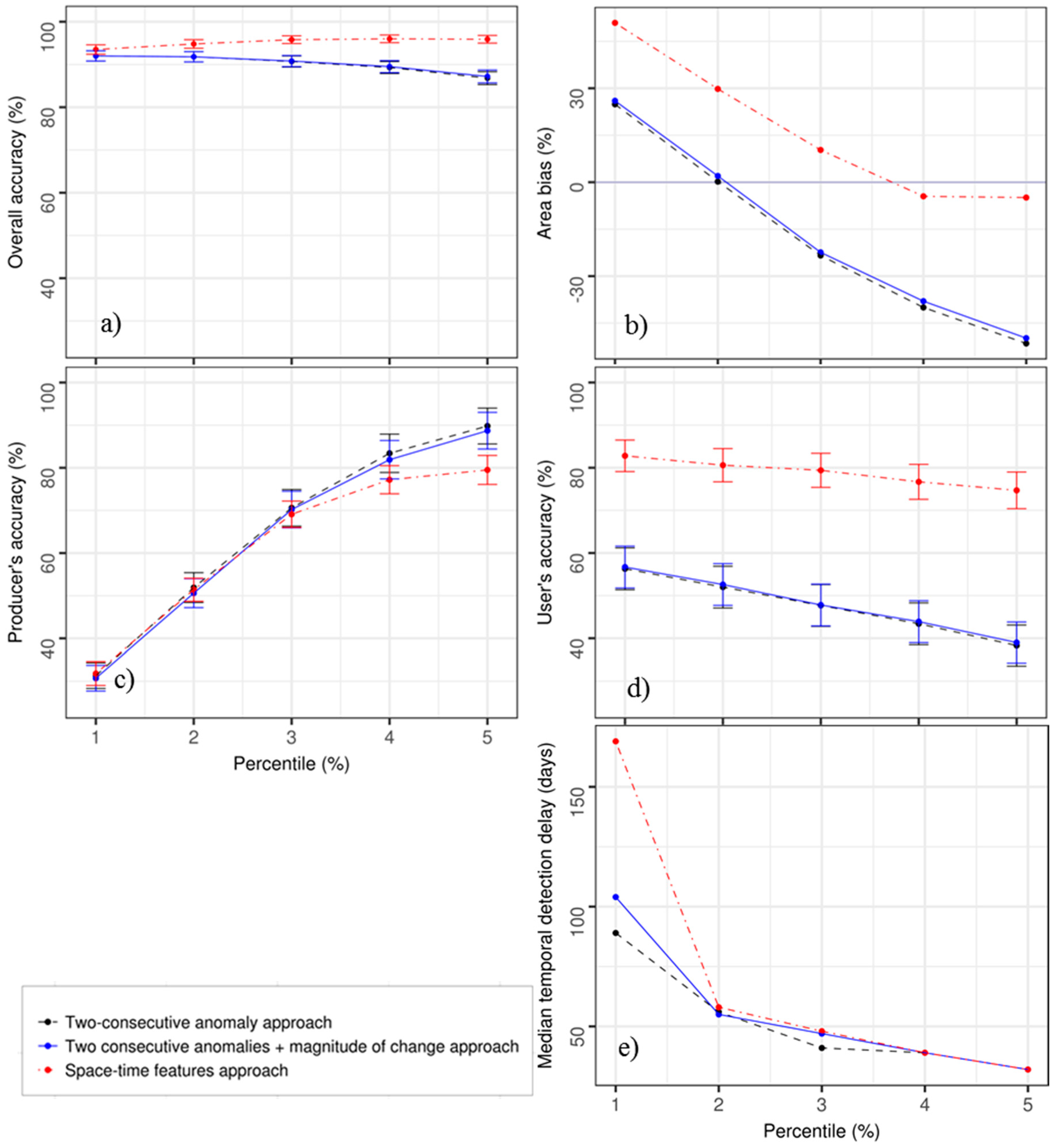
The space-time feature approach yielded the highest user’s accuracy across all the percentile thresholds (>70%, Figure 3d). More specifically, for each percentile threshold, the user’s accuracy achieved from the space-time feature approach was at least 26% higher than the user’s accuracy achieved either from a two-consecutive anomaly approach or from the magnitude of change approach. This gain in the user’s accuracy was particularly high (36.4%) when using the least strict percentile threshold (5th percentile). The difference in the user’s accuracy between the two-consecutive anomaly approach and the two consecutive anomalies + magnitude of change approach was marginal across all the percentile thresholds. Across all percentile thresholds, the user’s accuracy achieved from the two-consecutive anomaly approach and the two consecutive anomalies + magnitude of change approach was below 60%. Compared to the space-time feature approach, the two-consecutive anomaly approach and the two consecutive anomalies + magnitude of change approach achieved the higher producer’s accuracy when using the least strict percentile thresholds (4th and 5th percentile, Figure 3c), but the space-time feature approach achieved the highest overall accuracy (Figure 3a), and the lowest area bias (Figure 3b). More specifically, the producer’s accuracy for the space-time feature approach was about 9% lower than those of the two-consecutive anomaly approach and the two consecutive anomalies + magnitude of change approach when using the least strict percentile threshold. For all approaches, the least strict percentiles achieved the shortest temporal detection delay (32 days) and highest producer’s accuracy (>79%). For the space-time feature approach, the differences in the producer’s accuracy and median temporal detection delay between the most strict percentile threshold (5th percentile) and least strict percentile threshold (1st percentile) were 47.7% and 137 days, respectively. Figure 4 shows an example of a false detection, related to remnant clouds, which was accepted when using the two-consecutive anomaly approach and the magnitude of change approach, but rejected by the space-time feature approach.
4.2. The Effect of the Probability Threshold on Spatial Accuracy
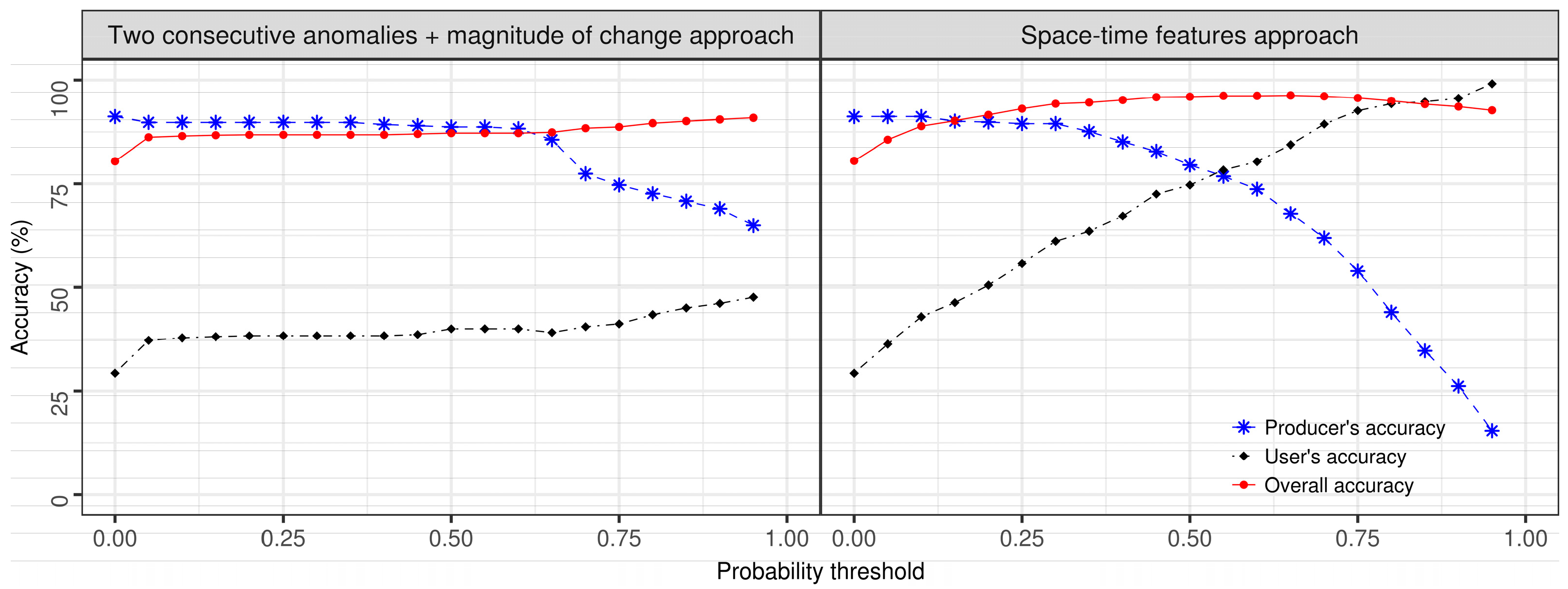
For the space-time approach, the user’s accuracy for map produced using the 5th percentile threshold increased by 69.8%, reaching 99.1% when increasing the probability threshold from 0 to 0.95. The producer’s accuracy decreased by 75.8 %, reaching 15.4%. The crossover point for the user’s and producer’s accuracy was approximately at the probability threshold of 0.55 (Figure 5). At this probability threshold, the user’s accuracy was 78.3% while the producer’s accuracy was 76.8%. In contrast, the user’s and producer’s accuracy did not reach the crossover point when using the two consecutive anomalies + magnitude of change approach (Figure 5). For this approach, the lowest area bias (17.3%) was achieved at the probability threshold of 0.95, and it was in favour of the producer’s accuracy. For the magnitude of change approach, the user’s accuracy only increased by 18.3%, reaching 47.6% when increasing the probability threshold from 0 to 0.95; and the producer’s accuracy decreased by 26.3%, reaching 64.3%.
4.3. Area Estimates for Disturbed Forest
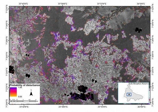
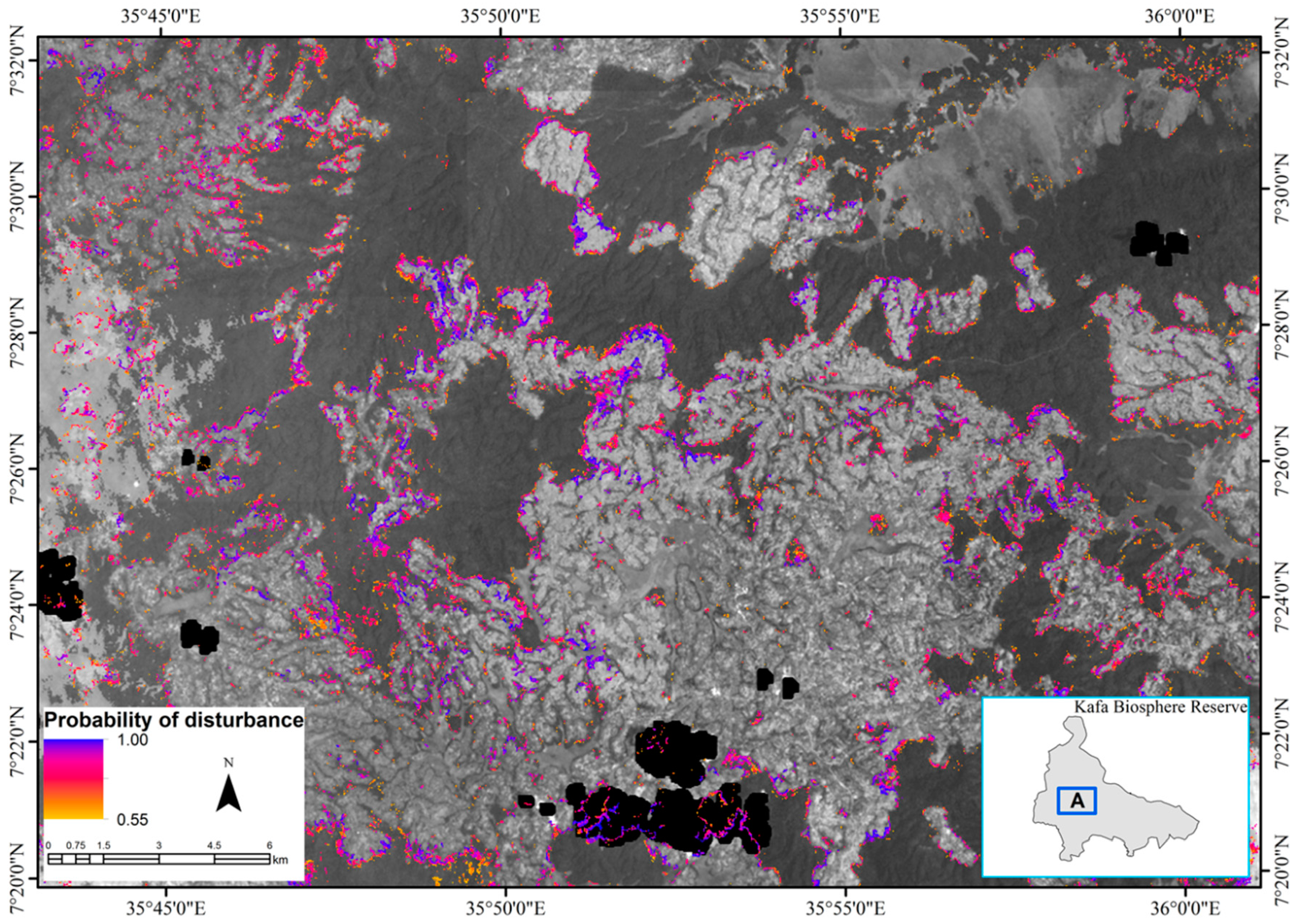
Using the map produced from the space-time feature approach, the 5th percentile threshold and probability threshold of 0.55 (Figure 6), we estimated that about 17,915 ha of forest in the UNESCO Kafa Biosphere Reserve has been disturbed between 2014 and 2016. The disturbances involved either full or partial removal of forest canopy. Disturbances were mainly concentrated at the edges of the forest (Figure 6).
4.4. Space-Time Features Important for Predicting Forest Disturbance
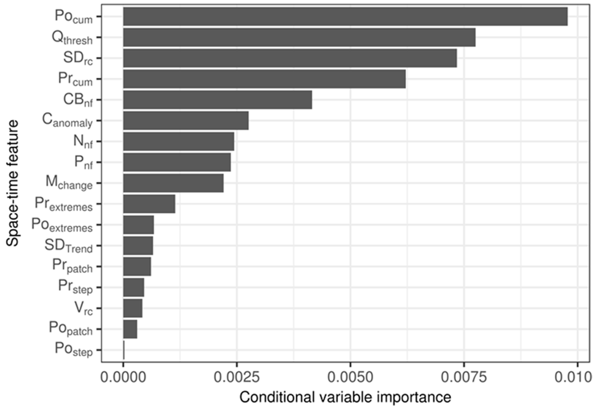
Our results show that cumulative sums of residuals for spatial variability (Pocum, and Prcum), the anomaly threshold for identifying anomalous observations (Qthresh), the variability in the reference cube of a local data cube (SDrc) and the number of non-forest pixels within the local data cube in the reference period (CBnf) were the most important predictors for forest disturbance (Figure 7). These space-time features were two times more important than consecutive negative anomalies (Canomaly) and the magnitude of change (Mchange).
5. Discussion
In this paper, we proposed the use of space-time features to improve forest change monitoring using Landsat time series. Space-time features are used to confirm forest disturbances when negative anomalies are detected in the pixel-time series. Our results show that using space-time features to confirm forest disturbances reduces false detections significantly, with minimal negative effect on producer’s accuracy for forest disturbance. Contrary to previous studies, our results also show that using two consecutive negative anomalies to confirm forest disturbances does not reduce false detections sufficiently even when using strict percentile thresholds to identify the anomalies. Instead of reducing false detections, strict percentile thresholds amplified the omission error, and led to a longer temporal detection delay. These results suggest that the criterion of two consecutive anomalies is not robust enough to reject false detection as previously thought [1,6,7]. Two consecutive anomalies might be sufficient in areas where forest disturbances occur at large scale and in an abrupt manner (e.g., [6,7]), but not sufficient when dealing with complex small-scale forest disturbances [13,20]. Our results also show that using the magnitude of change, in addition to two consecutive negative anomalies, to confirm forest disturbances does not reduce false detections sufficiently. The two consecutive anomalies + magnitude of change approach produced spatial and temporal accuracies largely similar to those of the two-consecutive anomalies approach. The false detections remained high despite using strict probability thresholds, implying that false detections also had high probability of disturbance when using magnitude of change as a predictor of forest disturbance. Overall, these findings suggest that temporal information alone might not be sufficient to reduce false detections, especially when aiming for accurate and timely detection of small-scale and gradual forest disturbances.
We observed that forest disturbances were mainly detected on the periphery of the forest. This pattern of forest disturbance is consistent with the findings of the previous studies [13,22] that mapped forest disturbances in this area using Landsat time series. The drivers of forest disturbance, especially expansion of small-holder agricultural areas and human settlements, are likely to occur on edges of the forest especially when there has been ongoing forest conservation and restoration activities in the area because it might be easier to illegally disturb forest edges than to clear new large intact forest area.
5.1. Importance of Space-Time Features for Accurate and Timely Detection of Forest Disturbances
Space-time features provided an opportunity to timely detect anomalies without amplifying false detections. This capacity to reject many false detections explains why the difference in the user’s accuracy between the maps produced using the least strict percentile threshold (5th percentile) and the maps produced using most strict percentile threshold (1st percentile) was only (8%). This difference was greater than 17% when using only two consecutive negative anomalies or magnitude of change to confirm forest disturbances. These results suggest that, although using less strict percentile thresholds may initially flag many pixels as potentially disturbed, a set of space-time features provides sufficient information to accurately discriminate false detections from real changes. At the same time, by using least strict percentile thresholds, we can reduce the omission error and the temporal detection delay. When aiming for the lowest area bias (1.5%), our spatial accuracies (overall accuracy = 96.2%, user’s accuracy = 76.8%, producer’s accuracy = 78.3%) were within the range of those reported in other studies that attempted to map forest disturbances at annual or sub-annual scales in recent years [6,7,9,11,13,37,38]. However, our high spatial accuracies were not achieved at the expense of temporal accuracy.
5.2. Important Space-Time Features for Forest Disturbance Predicting
Our analysis for conditional variable importance shows that space-time features which are related to spatial variability were the most important predictors for forest disturbances. More specifically, cumulative sum of residuals for spatial variability at the time step before the focal pixel is flagged as potentially disturbed, the anomaly threshold, the variability of the observations in the reference cube, and the cumulative sum of residuals for spatial variability at the time step the focal pixel is flagged as potentially disturbed were the most important predictors for forest disturbance. All these variables are computed using both spatial and temporal information, and are measuring spatio-temporal variability. The high importance of the variables related to spatio-temporal variability is not surprising because spatio-temporal variability is likely to increase once the forest becomes disturbed. The number of non-forest pixels within the local data cube was also an important predictor of forest disturbances. This is expected because new human-induced forest disturbance typically occurs closer to old disturbances in time and space [19]. Thus, negative anomalies detected at forest pixels which have spatial association with non-forest areas are most likely to signify forest disturbance. Magnitude of change and two consecutive negative anomalies, which are widely used to distinguish real changes from false detections [1,6,7,9,13], were not the strongest predictors for forest disturbance. Note, however, that our magnitude of change is computed differently from those used in other studies [9,13]. In our study area, forest disturbances are known to occur at a small-scale and in a gradual manner [13]. They may therefore have small magnitude of changes. This may explain why the magnitude of change was not a strong predictor of forest disturbance.
Although some space-time features were less important than others, it is important to highlight here that the importance of each space-time feature as a predictor for forest disturbance may vary from one area to another, depending on the nature of the forest disturbance. In areas where the forest is cleared on a large scale and involves sudden and full forest cover removal (e.g., [7,9,36]), the magnitude of change might be a strong predictor of forest disturbance. Nonetheless, the space-time feature approach is flexible because the probability of disturbance is calculated using a supervised machine learning algorithm [28]. However, an elaborate training data set to train the learning algorithm is needed to ensure the applicability of this approach to different forest areas. The requirement for training data is therefore disadvantageous because training data for forest disturbances are often lacking in many parts of the world [36], especially for small-scale forest disturbances which are difficult to acquire through visual interpretation of satellite images. Nonetheless, with the advent of community-based forest monitoring [39,40], observations on forest disturbances acquired through citizen science and local experts could be used for training purposes [20,22,40,41]. Availability of daily high-resolution images from nanosatellites sensors (e.g., Planet’s satellites) may also improve the acquisition of training data.
5.3. Space-Time Features Approach in the Era of Multi-Sensor Forest Disturbances
The approach of using space-time features that is presented in this paper is generic because the features we proposed here can be computed from image time series of any satellite sensor (e.g., Sentinel-2), including Synthetic Aperture Radar (SAR) sensors whose data has been widely used for forest monitoring in recent years [7,10,37,42,43]. Our approach can also be applied to other optical satellite data metrics. We can, for example, use all spectral bands, and extract space-time features from each spectral band. Such multi-spectral space-time feature can then be used to predict the probability of forest disturbances. In this way, we can concurrently exploit spatial, temporal and spectral information in satellite data to accurately and timely map forest disturbance. It should be noted, however, that a clear understanding of how reflectance in each spectral channel reacts to forest disturbance is needed to extract consistent and meaningful space-time features.
6. Conclusions
This paper demonstrated that using space-time features extracted from Landsat NDVI data cubes to confirm forest disturbance increases the capacity to reject many false detections, without compromising the temporal accuracy. The use of space-time features is based on the idea that forest disturbances, by default, are spatio-temporal processes, hence information on spatio-temporal association and variability in satellite time series should be considered to accurately and efficiently detect forest disturbances. The following space-time features were the strongest predictors for forest disturbance: (1) the change in spatio-temporal variability, (2) spatio-temporal association with non-forest, and (3) variability in the reference period. Magnitude of change and two consecutive negative anomalies, which are widely used to distinguish real changes from false detections, were not the main predictors of forest disturbance. These findings indicate that space-time features have potential to improve the detection of forest disturbances, especially small-scale and gradual forest disturbances whose magnitude of change is often small. Detection of small scale forest disturbances may further improve when using satellite sensors, like Sentinel-2, that provide increased spatial and temporal details.
Acknowledgments
The work of Eliakim Hamunyela and Jan Verbesselt was funded by the European Space Agency (ESA) ForMoSa project—Forest Degradation Monitoring with Satellite Data Project (grant agreement 5160957022). The work of Johannes Reiche and Martin Herold was funded by the European Commission Horizon 2020 BACI project (grant agreement 640176).
Author Contributions
Eliakim Hamunyela, Johannes Reiche, Jan Verbesselt and Martin Herold conceived and designed the study; Eliakim Hamunyela performed the experiments, analysed the data, and wrote the paper.
Conflicts of Interest
The authors declare no conflict of interest.
References
- Zhu, Z.; Woodcock, C.E.; Olofsson, P. Continuous monitoring of forest disturbance using all available Landsat imagery. Remote Sens. Environ. 2012, 122, 75–91. [Google Scholar] [CrossRef]
- Xin, Q.; Olofsson, P.; Zhu, Z.; Tan, B.; Woodcock, C.E. Toward near real-time monitoring of forest disturbance by fusion of MODIS and Landsat data. Remote Sens. Environ. 2013, 135, 234–247. [Google Scholar] [CrossRef]
- Zhu, Z.; Woodcock, C.E. Continuous change detection and classi fi cation of land cover using all available Landsat data. Remote Sens. Environ. 2014, 144, 152–171. [Google Scholar] [CrossRef]
- Hilker, T.; Wulder, M.A.; Coops, N.C.; Seitz, N.; White, J.C.; Gao, F.; Masek, J.G.; Stenhouse, G. Generation of dense time series synthetic Landsat data through data blending with MODIS using a spatial and temporal adaptive re fl ectance fusion model. Remote Sens. Environ. 2009, 113, 1988–1999. [Google Scholar] [CrossRef]
- Verbesselt, J.; Zeileis, A.; Herold, M. Near real-time disturbance detection using satellite image time series. Remote Sens. Environ. 2012, 123, 98–108. [Google Scholar] [CrossRef]
- Hamunyela, E.; Verbesselt, J.; De Bruin, S.; Herold, M. Monitoring deforestation at sub-annual scales as extreme events in Landsat data cubes. Remote Sens. 2016, 8, 651. [Google Scholar] [CrossRef]
- Reiche, J.; de Bruin, S.; Hoekman, D.; Verbesselt, J.; Herold, M. 1 A bayesian approach to combine Landsat and ALOS PALSAR time series for near real-time deforestation detection. Remote Sens. 2015, 7, 4973–4996. [Google Scholar] [CrossRef]
- Hansen, M.C.; Krylov, A.; Tyukavina, A.; Potapov, P.V.; Turubanova, S.; Zutta, B.; Ifo, S.; Margono, B.; Stolle, F.; Moore, R. Humid tropical forest disturbance alerts using Landsat data. Environ. Res. Lett. 2016, 11, 34008. [Google Scholar] [CrossRef]
- Hamunyela, E.; Verbesselt, J.; Herold, M. Using spatial context to improve early detection of deforestation from Landsat time series. Remote Sens. Environ. 2016, 172, 126–138. [Google Scholar] [CrossRef]
- Reiche, J.; Hamunyela, E.; Verbesselt, J.; Hoekman, D.; Herold, M. Improving near-real time deforestation monitoring in tropical dry forests by combining dense Sentinel-1 time series with Landsat and ALOS-2 PALSAR-2. Remote Sens. Environ. 2017. submitted. [Google Scholar]
- Dutrieux, L.P.; Verbesselt, J.; Kooistra, L.; Herold, M. Monitoring forest cover loss using multiple data streams, a case study of a tropical dry forest in Bolivia. ISPRS J. Photogramm. Remote Sens. 2015, 107, 112–125. [Google Scholar] [CrossRef]
- Vermote, E.; Justice, C.O.; Bréon, F. Towards a Generalized Approach for Correction of the BRDF Effect in MODIS Directional Reflectances. IEEE Trans. Geosci. Remote Sens. 2009, 47, 898–908. [Google Scholar] [CrossRef]
- Devries, B.; Verbesselt, J.; Kooistra, L.; Herold, M. Robust monitoring of small-scale forest disturbances in a tropical montane forest using Landsat time series. Remote Sens. Environ. 2015, 161, 107–121. [Google Scholar] [CrossRef]
- Huang, C.; Goward, S.N.; Schleeweis, K.; Thomas, N.; Masek, J.G.; Zhu, Z. Dynamics of national forests assessed using the Landsat record: Case studies in eastern United States. Remote Sens. Environ. 2009, 113, 1430–1442. [Google Scholar] [CrossRef]
- Fisher, B. African exception to drivers of deforestation. Nat. Geosci. 2010, 3, 375–376. [Google Scholar] [CrossRef]
- Schultz, M.; Clevers, J.G.P.W.; Carter, S.; Verbesselt, J.; Avitabile, V.; Vu, H.; Herold, M. Performance of vegetation indices from Landsat time series in deforestation monitoring. Int. J. Appl. Earth Obs. Geoinf. 2016, 52, 318–327. [Google Scholar] [CrossRef]
- Tyukavina, A.; Stehman, S.V.; Potapov, P.V.; Turubanova, S.A.; Baccini, A.; Goetz, S.J.; Laporte, N.T.; Houghton, R.A.; Hansen, M.C. National-scale estimation of gross forest aboveground carbon loss: A case study of the Democratic Republic of the Congo. Environ. Res. Lett. 2013, 8, 044039. [Google Scholar] [CrossRef]
- Zscheischler, J.; Mahecha, M.D.; Harmeling, S.; Reichstein, M. Detection and attribution of large spatiotemporal extreme events in Earth observation data. Ecol. Inform. 2013, 15, 66–73. [Google Scholar] [CrossRef]
- Alves, D.S. Space-time dynamics of deforestation in Brazilian Amazônia. Int. J. Remote Sens. 2002, 23, 2903–2908. [Google Scholar] [CrossRef]
- Pratihast, A.K.; DeVries, B.; Avitabile, V.; de Bruin, S.; Kooistra, L.; Tekle, M.; Herold, M. Combining satellite data and community-based observations for forest monitoring. Forests 2014, 5, 2464–2489. [Google Scholar] [CrossRef]
- Dresen, E.; Devries, B.; Herold, M.; Verchot, L.; Müller, R. Fuelwood savings and carbon emission reductions by the use of improved cooking stoves in an afromontane forest, Ethiopia. Land 2014, 3, 1137–1157. [Google Scholar] [CrossRef]
- Devries, B.; Pratihast, A.K.; Verbesselt, J.; Kooistra, L.; Herold, M. Characterizing forest change using community-based monitoring data and Landsat time series. PLoS ONE 2016, 11, e0147121. [Google Scholar] [CrossRef] [PubMed]
- Tucker, C.J. Red and photographic infrared linear combinations for monitoring vegetation. Remote Sens. Environ. 1979, 150, 127–150. [Google Scholar] [CrossRef]
- Rouse, J.W.; Haas, R.H.; Schell, J.A.; Deering, D.W. Monitoring Vegetation Systems in the Great Plains with ERTS. In Proceedings of the Third Earth Resource Technology Satellite (ERTS) Symposium, Greenbelt, MD, USA, 10–14 December 1973; NASA: Washington, DC, USA; pp. 309–317. [Google Scholar]
- Masek, J.G.; Vermote, E.F.; Saleous, N.E.; Wolfe, R.; Hall, F.G.; Huemmrich, K.F.; Gao, F.; Kutler, J.; Lim, T. A Landsat surface reflectance dataset for North America, 1990–2000. IEEE Geosci. Remote Sens. Lett. 2006, 3, 68–72. [Google Scholar] [CrossRef]
- Vermote, E.; Justice, C.; Claverie, M.; Franch, B. Preliminary analysis of the performance of the Landsat 8/OLI land surface re fl ectance product. Remote Sens. Environ. 2016, 185, 46–56. [Google Scholar] [CrossRef]
- Zhu, Z.; Woodcock, C.E. Object-based cloud and cloud shadow detection in Landsat imagery. Remote Sens. Environ. 2012, 118, 83–94. [Google Scholar] [CrossRef]
- Breiman, L.E.O. Random Forests. Mach. Learn. 2001, 45, 5–32. [Google Scholar] [CrossRef]
- Strobl, C.; Boulesteix, A.; Kneib, T.; Augustin, T.; Zeileis, A. Conditional variable importance for random forests. BMC Bioinform. 2008, 9, 307. [Google Scholar] [CrossRef] [PubMed]
- Ichoku, C.; Chu, D.A.; Mattoo, S.; Kaufman, Y.J.; Remer, L.A.; Tanre, D.; Slutsker, I.; Holben, B.N. A spatio-temporal approach for global validation and analysis of MODIS aerosol products. Geophys. Res. Lett. 2002, 29, 1616. [Google Scholar] [CrossRef]
- Glasbey, C.A.; Graham, R.; Hunter, A.G.M. Spatio-temporal variability of solar energy across a region: A statistical modelling approach. Sol. Energy Vol. 2001, 70, 373–381. [Google Scholar] [CrossRef]
- Uddstrom, M.J.; Oien, N.A. On the use of high-resolution satellite data to describe the spatial and temporal variability of sea surface temperatures in the New Zealand region. J. Geophys. Res. 1999, 104, 20729–20751. [Google Scholar] [CrossRef]
- Stehman, S.V. Sampling designs for accuracy assessment of land cover. Int. J. Remote Sens. 2009, 30, 5243–5272. [Google Scholar] [CrossRef]
- Olofsson, P.; Foody, G.M.; Herold, M.; Stehman, S.V.; Woodcock, C.E.; Wulder, M.A. Good practices for estimating area and assessing accuracy of land change. Remote Sens. Environ. 2014, 148, 42–57. [Google Scholar] [CrossRef]
- Stehman, S.V. Impact of sample size allocation when using stratified random sampling to estimate accuracy and area of land-cover change. Remote Sens. Lett. 2012, 3, 111–120. [Google Scholar] [CrossRef]
- Cohen, W.B.; Yang, Z.; Kennedy, R. Detecting trends in forest disturbance and recovery using yearly Landsat time series: 2. TimeSync—Tools for calibration and validation. Remote Sens. Environ. 2010, 114, 2911–2924. [Google Scholar] [CrossRef]
- Reiche, J.; Verbesselt, J.; Hoekman, D.; Herold, M. Fusing Landsat and SAR time series to detect deforestation in the tropics. Remote Sens. Environ. 2015, 156, 276–293. [Google Scholar] [CrossRef]
- Grogan, K.; Dirk, P.; Hostert, P.; Kennedy, R.; Fensholt, R. Cross-border forest disturbance and the role of natural rubber in mainland Southeast Asia using annual Landsat time series. Remote Sens. Environ. 2015, 169, 438–453. [Google Scholar] [CrossRef]
- Pratihast, A.K.; Herold, M.; Avitabile, V.; de Bruin, S.; Bartholomeus, H.; Souza, C.M.; Ribbe, L. Mobile devices for community-based REDD+ monitoring: A case study for Central Vietnam. Sensors 2012, 13, 21–38. [Google Scholar] [CrossRef] [PubMed]
- Pratihast, A.K.; Devries, B.; Avitabile, V.; Bruin, S. De; Herold, M. Design and implementation of an interactive web-based near real-time forest monitoring system. PLoS ONE 2016, 11, e0150935. [Google Scholar] [CrossRef] [PubMed]
- See, L.; Fritz, S.; Victoria, D.G. Beyond sharing Earth observations. Nature 2014, 514, 168. [Google Scholar] [CrossRef] [PubMed]
- Lehmann, E.A.; Caccetta, P.A.; Zhou, Z.; Mcneill, S.J.; Wu, X.; Mitchell, A.L. Joint processing of Landsat and ALOS-PALSAR data for forest mapping and monitoring. IEEE Trans. Geosci. Remote Sens. 2012, 50, 55–67. [Google Scholar] [CrossRef]
- Lehmann, E.A.; Caccetta, P.; Lowell, K.; Mitchell, A.; Zhou, Z.; Held, A.; Milne, T.; Tapley, I. SAR and optical remote sensing: Assessment of complementarity and interoperability in the context of a large-scale operational forest monitoring system. Remote Sens. Environ. 2015, 156, 335–348. [Google Scholar] [CrossRef]
Figure 1.
Overview of the UNESCO Kafa Biosphere Reserve located in southwest of Ethiopia. Areas in green represent the benchmark forest map. The benchmark forest map was generated using a supervised maximum likelihood classifier.
Figure 1.
Overview of the UNESCO Kafa Biosphere Reserve located in southwest of Ethiopia. Areas in green represent the benchmark forest map. The benchmark forest map was generated using a supervised maximum likelihood classifier.

Figure 2.
The workflow for this study.

Figure 3.
Overall accuracy (a); area bias (b); producer’s accuracy (c); user’s accuracy (d); and median temporal detection delay (e) for forest disturbances detected in the UNESCO Kafa Biosphere Reserve between 2014 and 2016 from Landsat NDVI time series. Forest disturbances were confirmed using three approaches: the two-consecutive anomalies approach, the two consecutive anomalies + magnitude of change approach and the space-time feature approach. The accuracies are shown as a function for the percentile thresholds for declaring anomalous observations in local data cubes. The vertical bars in (a,c,d) indicate the 95% confidence interval.

Figure 4.
An example of a false detection (red dotted line), related to remnant clouds, which was rejected (probability of disturbance = 0.13) when using the space-time features. The probability of disturbance was 0.51 when only using the magnitude of change to predict forest disturbance. The magnitude of change was −0.22. The red dot represents the pixel (location: 7°30′5.042″N, 36°1′30.959″E) whose time series is shown, and the black areas in the image chips represent areas which were masked as clouds or cloud shadow using CFmask. Image chips which were covered completely with no data are skipped.

Figure 5.
Overall accuracy, producer’s accuracy and user’s accuracy for forest disturbances detected in the UNESCO Kafa Biosphere Reserve between 2014 and 2016 from Landsat NDVI time series using the 5th percentile while changing the probability threshold for accepting two consecutive negative anomalies as forest disturbance.

Figure 6.
An example of forest disturbances detected in the UNESCO Kafa Biosphere Reserve between 2014 and 2016 from Landsat NDVI time series (insert A). The probability disturbance was calculated using the space-time features extracted from Landsat NDVI data cubes based on the 5th percentile threshold and 0.55 probability threshold. The base image is the surface reflectance in the red channel (Band 4) for Landsat-8/OLI acquired on 10 March 2016. The black patches represent areas masked for clouds and cloud shadows.

Figure 7.
Conditional variable importance for each space-time feature used to predict forest disturbances in the UNESCO Kafa Biosphere Reserve from data cubes of Landsat normalised difference vegetation index (NDVI) time series. Training data (n = 1311) was used to determine the conditional variable importance.


Table 1.
Space-time features extracted from local data cubes for Landsat NDVI time series to predict the probability of forest disturbances given two consecutive negative anomalies at a particular pixel. The spatial extent of the local data cube was 15 by 15 Landsat pixels. T1 refers to the time step where the first negative anomaly of the two consecutive negative anomalies is detected, whereas T2 is the time step for the second negative anomaly. The space-time features are grouped by category in the table.
| Category | Feature | Acronym | Data Type | Explanation |
|---|---|---|---|---|
| Temporal | Consecutive anomalies | Canomaly | Discrete-Numeric | Number of consecutive negative anomalies. Here, we used two consecutive negative anomalies |
| Magnitude of change | Mchange | Continuous | Magnitude of change calculated by subtracting the anomaly threshold from the second anomaly at T2 | |
| Spatial | Number of non-forest pixels in the reference period | CBnf | Discrete-Numeric | Number of pixels within the local data cube which have been masked as non-forest in the reference period |
| Presence of non-forest neighbours | Nnf | Binary (yes = 1, no = 0) | Indicates whether any of the 8-connected neighbours for the focal pixel is already non-forest in the reference period | |
| Number non-forest neighbours | Pnf | Discrete-Numeric | Number of the 8-connected neighbours for the focal pixel which are already non-forest in the reference period | |
| Presence of neighbours with negative anomalies at T1 | Prstep | Binary (yes = 1, no = 0) | Indicates whether any of the 8-connected neighbours for the focal pixel also experienced negative anomalies at T1 | |
| Number of neighbours with negative anomalies at T1 | Prpatch | Discrete-Numeric | Number of 8-connected neighbours for focal pixel which also experienced negative anomalies at T1 | |
| Number of pixels in the local data cube with negative anomalies at T1 | Prextremes | Discrete-Numeric | Number of pixels in the local data cube which also experienced negative anomalies at T1 | |
| Presence of neighbours with negative anomalies at T2 | Postep | Binary (yes = 1, no = 0) | Indicates whether any of the 8-connected neighbours of the focal pixel is also experiencing negative anomalies at T2 | |
| Number of neighbours with anomalies T2 | Popatch | Discrete-Numeric | Number of 8-connected neighbours of the focal pixel which are also experiencing negative anomalies at T2 | |
| Number of pixels with negative anomalies in the local data cube at T2 | Poextremes | Discrete-Numeric | Number of pixels in local data cube with negative anomalies at T2 | |
| Spatio-temporal | Cumulative sum of residuals for spatial variability at T2 | Pocum | Continuous | Cumulative sum of residuals for spatial variability at T2. Calculated following these steps: (1) calculate spatial variation (standard deviation) at each time step of the time series; (2) calculate the temporal mean of spatial variation; (3) subtract the temporal mean of spatial variation from spatial variation at each time step |
| Cumulative sum of residuals for spatial variability at T1 | Prcum | Continuous | Cumulative sum of residuals for spatial variability at T1. Calculated in same way as Pocum above | |
| Anomaly threshold | Qthresh | Continuous | Threshold for identifying negative anomalies, computed from the local data cube over the reference period, corresponding to the specified percentile (e.g., 5th percentile) | |
| Variability of observations in the local data cube in the reference period | SDrc | Continuous | Standard deviation of the observations in the reference period of a local data cube | |
| Temporal linear trend in spatial variability | SDTrend | Continuous | Temporal linear trend in spatial variability, quantified using a linear model | |
| Number of observations in local data cube over the reference period | Vrc | Discrete- Numeric | Number of valid observations in the local data cube over the reference period |
Table 2.
Area proportions, number of pixels and allocated sample size for each stratum.
| Stratum | No. of Pixels | Area Proportion | No. of Samples |
|---|---|---|---|
| No change I | 2,694,771 | 0.888 | 1443 |
| No Change II | 261,204 | 0.086 | 500 |
| Change I | 71,167 | 0.023 | 200 |
| Change II | 7667 | 0.003 | 200 |
| Total | 3,034,809 | 1 | 2343 |
© 2017 by the authors. Licensee MDPI, Basel, Switzerland. This article is an open access article distributed under the terms and conditions of the Creative Commons Attribution (CC BY) license (http://creativecommons.org/licenses/by/4.0/).
Share and Cite
MDPI and ACS Style
Hamunyela, E.; Reiche, J.; Verbesselt, J.; Herold, M. Using Space-Time Features to Improve Detection of Forest Disturbances from Landsat Time Series. Remote Sens. 2017, 9, 515. https://doi.org/10.3390/rs9060515
AMA Style
Hamunyela E, Reiche J, Verbesselt J, Herold M. Using Space-Time Features to Improve Detection of Forest Disturbances from Landsat Time Series. Remote Sensing. 2017; 9(6):515. https://doi.org/10.3390/rs9060515
Chicago/Turabian StyleHamunyela, Eliakim, Johannes Reiche, Jan Verbesselt, and Martin Herold. 2017. "Using Space-Time Features to Improve Detection of Forest Disturbances from Landsat Time Series" Remote Sensing 9, no. 6: 515. https://doi.org/10.3390/rs9060515
Note that from the first issue of 2016, this journal uses article numbers instead of page numbers. See further details here.